Visualize Surface
14 Feb 2015To install Systematic Investor Toolbox (SIT) please visit About page.
The smoothness, convexity, of objective function is critical to success of optimization.
Visualizing an objective function is an easy and convenient way to check for smoothness.
For example, let’s check the Ulcer Index , an alternative measure of risk, similar to Standard Deviation.
If the Ulcer Index is a smooth function it can easily be used in optimization using for example a non-linear solver.
#*****************************************************************
# Simulate data for 3 asset universe
#*****************************************************************
library(SIT)
load.packages('quantmod')

S = c(100,105,20) # spot prices
r = c(0.05, 0.11,0.1) # expected returns
sigma = c(0.11,0.16,0.27) # expected standard deviations matrix
rho12 = 0.63 # correlation between first and second assets
rho13 = 0.2 # correlation between first and third assets
rho23 = 0.89 # correlation between second and third assets

# construct correlation matrix
rho = matrix(1,nr=3,nc=3)
rho[upper.tri(rho)] = c(rho12,rho13,rho23)
rho = rho+t(rho)-1

# make sure correlation matrix is positive defined matrix
load.packages('Matrix')
rho = as.matrix(nearPD(rho, T)$mat)


# simulate 100 days
periods = 0:100/252
cov.matrix = sigma%*%t(sigma) * rho
# check that covariance matrix is positive defined, i.e. all eigenvalues > 0
#eigen(cov.matrix)
prices = asset.paths(S, r, cov.matrix, 1, periods = periods)
  prices = t(prices[,,1])

#*****************************************************************
# Look at Simulated prices
#*****************************************************************
xts.prices = make.xts(prices, seq(Sys.Date()-100, Sys.Date(), 1))
  colnames(xts.prices) = paste('Asset', 1:3)
plota.matplot(scale.one(xts.prices),main='Asset Perfromance')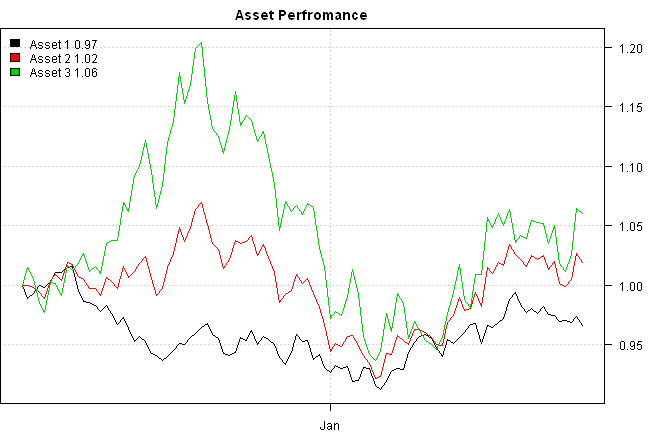
#*****************************************************************
# Compute Ulcer Index
#*****************************************************************
prices = scale.one(prices)

temp = seq(0,100,5)
choices = expand.grid(x = temp, y = temp) / 100

z = apply(choices,1, function(x) {
	if(sum(x) > 1) NA
	else
 	last(ulcer.index(x[1]*prices[,1] + x[2]*prices[,2] + (1-sum(x))*prices[,3]))
}
)
z = matrix(z,len(temp))

#*****************************************************************
# Visualize Surface - static 3D plot
#*****************************************************************
persp(temp, temp, z,col='green',xlab='x',ylab='y',zlab='ulcer',theta=30,phi=30,expand=0.5)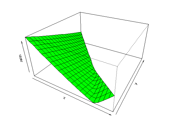
Above code creates a static surface plot that is hard to investigate.
To create interactive 3D plot that can be rotated with mouse, please use:
#*****************************************************************
# Visualize Surface - interactive 3D plot, use mouse to rotate
#*****************************************************************
load.packages('rgl')
persp3d(temp, temp, z,col='green',xlab='x',ylab='y',zlab='ulcer')
The Ulcer Index looks smooth and is a suitable candidate for optimization.
(this report was produced on: 2015-02-15)