Benchmark Plus
14 Apr 2016To install Systematic Investor Toolbox (SIT) please visit About page.
The overlay strategy is the market neutral strategy that can be applied to benchmark to improve benchmark’s performance. The new strategy weights are equal to benchmark weights plus the overlay weights.
Below I will present a very simple example. The Benchmark portfolio is a market cap weighted country portfolio. The Overlay portfolio is long the top five momentum countries and is short the bottom five momentum countries. The Benchmark Plus portfolio is the Benchmark portfolio combined with the Overlay portfolio.
I will use the Betting Against Beta: Equity Factors, Monthly historical data set to download:
- market excess returns,
- lagged market capitalization,
- risk free rate
To construct the Benchmark portfolio, a market cap weighted country portfolio, returns please multiply market returns by normalized market capitalization weights
#*****************************************************************
# construct market cap weighted benchmark, no need to lag market.cap; it is t-1
#******************************************************************
benchmark.weight = data$market.cap / rowSums(data$market.cap)
benchmark.ret = xts(rowSums(benchmark.weight * data$market), dates)
benchmark.equity = cumprod(1 + benchmark.ret)
To construct the Overlay portfolio, a market neutral portfolio that is long the top five momentum countries and is short the bottom five momentum countries, please first ensure that overlay portfolio weights satisfy that Benchmark portfolio weight plus the Overlay portfolio weight are with in 0 and 1. Next normalize the Overlay portfolio weights to sum up to 0. This insures the Benchmark Plus portfolio is fully invested.
#*****************************************************************
# construct overlay
#******************************************************************
# rank countries based on 1 month return, overweight top 5 and underweight bottom 5
mom = mlag(data$mom)

# make sure that overlay + benchmark weights is always from 0 to 1 and sums up to 1
long.weight = iif(ntop(mom,5) > (1 - benchmark.weight), 1 - benchmark.weight, ntop(mom,5))
short.weight = iif(ntop(mom,5,F) > benchmark.weight, benchmark.weight, ntop(mom,5,F))

# scale long and short weights to offset each other
overlay.weight =  rowSums(short.weight)* long.weight / rowSums(long.weight) - short.weight
	overlay.weight[1,] = 0
Finally, to construct the Benchmark Plus portfolio, the Benchmark portfolio combined with the Overlay portfolio, returns please multiply market returns by combined Benchmark portfolio weights and Overlay portfolio weights.
#*****************************************************************
# construct strategy = benchmark + overlay
#******************************************************************
# please note weights are already lagged
strategy.weight = benchmark.weight + overlay.weight
strategy.ret = xts(rowSums(strategy.weight * data$market), dates)
strategy.equity = cumprod(1 + strategy.ret)
Now, I will construct:
- annualized tracking error - the annualized active risk
- annualized information ratio - the annualized alpha divided by annualized active risk
#*****************************************************************
# compute descriptive statistics
#******************************************************************
# make sure weights add up
# range(rowSums(abs(strategy.weight)))

tracking.error = sqrt(12) * sd(strategy.ret - benchmark.ret)

alpha = 12*(mean(strategy.ret) - mean(benchmark.ret))

information.ratio = alpha / tracking.error

print(data.frame(alpha, tracking.error, information.ratio))| alpha | tracking.error | information.ratio |
|---|---|---|
| 0.0160963 | 0.0309904 | 0.519397 |
I get 0.5 annualized information ratio and 3% tracking error; not a bad result for such a simple system.
Following are the descriptive statistics for both portfolios and historical performance chart.
#*****************************************************************
# Create model and Reports
#******************************************************************
models = list()
models$benchmark = lst(ret = benchmark.ret, equity=benchmark.equity, weight=benchmark.weight)
models$strategy = lst(ret = strategy.ret, equity=strategy.equity, weight=strategy.weight)

plotbt(models, plotX = T, log = 'y', LeftMargin = 3, main = NULL)
	mtext('Cumulative Performance', side = 2, line = 1)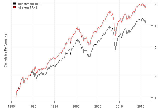
print(plotbt.strategy.sidebyside(models, make.plot=F, return.table=T,perfromance.fn = engineering.returns.kpi))| benchmark | strategy | |
|---|---|---|
| Period | Jan1986 - Feb2016 | Jan1986 - Feb2016 |
| Cagr | 8.25 | 9.97 |
| Sharpe | 0.59 | 0.68 |
| DVR | 0.52 | 0.61 |
| R2 | 0.88 | 0.89 |
| Volatility | 15.61 | 15.77 |
| MaxDD | -54.46 | -55.23 |
| Exposure | 100 | 100 |
Following are the transition map plots for both strategies. There is a bit of noise in the Benchmark Plus strategy due to momentum portfolio changes.
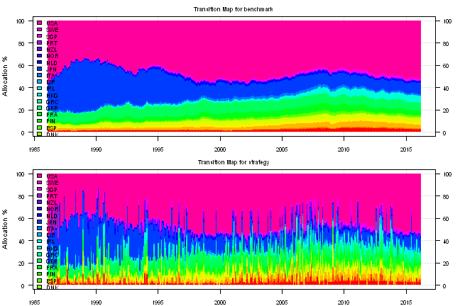
Overall, the Benchmark Plus strategy maintains a similar risk profile as the original Benchmark strategy and is able improve performance. I think for such a simple strategy it works quite well.
For your convenience, the 2016-04-14-Benchmark-Plus post source code.