RFinance 2016
15 May 2016To install Systematic Investor Toolbox (SIT) please visit About page.
The code below is used in the Tax Aware Backtest Framework presentation at RFinance 2016 .
First an Artificial Example demonstrates the impact of taxes by exploring the difference between long-term and short-term capital gain taxes.
Suppose we have two identical assets, two clones of SPY for this example. Consider an annually re-balanced strategy that does 100% turnover by moving from one SPY clone to another.
The OneYear strategy does the re-balance at the end of the year, hence it is subject to the short-term capital gain tax. The OneYearOneDay strategy does re-balance at one year plus one day, hence it is subject to the long-term capital gain tax.
#*****************************************************************
# Load historical data
#*****************************************************************
library(SIT)
library(quantmod)

tickers = 'SPY'

data = env()
getSymbols.extra(tickers, src = 'yahoo', from = '1970-01-01', env = data, auto.assign = T)
	# clone SPY
	data$SPY1 = data$SPY

	# compute implied dividends and splits from adjusted quotes
	bt.unadjusted.add.div.split(data, infer.div.split.from.adjusted=T)

bt.prep(data, align='remove.na', fill.gaps = T, dates='::2016:05:13')

#*****************************************************************
# Setup
#*****************************************************************
prices = data$prices
	nperiods = nrow(prices)
period.ends = date.ends(prices,'years')

models = list()

one.year = date.ends.n(prices, 365, period.ends[1])
one.year.one.day = date.ends.n(prices, 365, period.ends[1], less = F)

weight = matrix(c(0,1,1,0),nr=100,nc=2, byrow=T) # 100% turnover

#*****************************************************************
# Before Tax
#*****************************************************************
models = list()

# must reinvest dividends right away to match performance between 2 strategies
dividend.control = list(invest = 'rebalance')

data$weight[] = NA
	data$weight[one.year,] = weight[1:len(one.year),]
models$BeforeTax = bt.run.share.ex(data, clean.signal=F, silent=T, adjusted = F,
	dividend.control = dividend.control)

data$weight[] = NA
	data$weight[one.year.one.day,] = weight[1:len(one.year.one.day),]
models$BeforeTax = bt.run.share.ex(data, clean.signal=F, silent=T, adjusted = F,
	dividend.control = dividend.control)


#*****************************************************************
# After Tax
#*****************************************************************
tax.control = default.tax.control()
cashflow.control = list(
	taxes = list(
		cashflows = event.at(prices, period.ends = custom.date.bus('1 day in April', prices), offset=0),
		cashflow.fn = tax.cashflows,
		invest = 'update', # minimally update portfolio to have cash to pay taxes
		type = 'fee.rebate'
	)
)

data$weight[] = NA
	data$weight[one.year,] = weight[1:len(one.year),]
models$OneYearTax = bt.run.share.ex(data, clean.signal=F, silent=T, adjusted = F,
	tax.control=tax.control, cashflow.control = cashflow.control)

data$weight[] = NA
	data$weight[one.year.one.day,] = weight[1:len(one.year.one.day),]
models$OneYearOneDayTax = bt.run.share.ex(data, clean.signal=F, silent=T,  adjusted = F,
	tax.control=tax.control, cashflow.control = cashflow.control)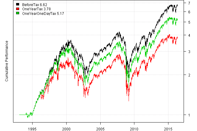
| BeforeTax | OneYearTax | OneYearOneDayTax | |
|---|---|---|---|
| Cagr | 8.4 | 5.9 | 7.3 |
| TaxImpact | 29.8 | 13.1 | |
| Detail | =1 - 5.9/8.4 | =1 - 7.3/8.4 |
Please note that implied tax rate is lower then tax rate specified in the default.tax.control
function. This is due to the two Bear markets during the test. The losses incurred during the
Bear markets are later on offset with gains during consequent Bull markets.
In reality the impact of taxes is not that profound. Next, let’s study a more realistic example.
Consider a monthly re-balanced strategy that allocates across 9 sector ETFs using either equal weight or minimum variance weighing schemes.
#*****************************************************************
# Load historical data
#*****************************************************************
library(SIT)
library(quantmod)

tickers = 'XLY,XLP,XLE,XLF,XLV,XLI,XLB,XLK,XLU'

data = env()
getSymbols.extra(tickers, src = 'yahoo', from = '1970-01-01', env = data, auto.assign = T)

	# compute implied dividends and splits from adjusted quotes
	bt.unadjusted.add.div.split(data, infer.div.split.from.adjusted=T)

bt.prep(data, align='remove.na', fill.gaps = T, dates='::2016:05:13')

#*****************************************************************
# Setup
#*****************************************************************
prices = bt.apply(data, Ad)
  n = ncol(prices)
  nperiods = nrow(prices)

period.ends = date.ends(data$prices,'months')

#*****************************************************************
# Strategy
#******************************************************************
obj = portfolio.allocation.helper(data$prices, period.ends = period.ends, lookback.len = 250,
	min.risk.fns = list(
		EqWt=equal.weight.portfolio,
		MinVar=min.var.portfolio
	),
	silent=T
)

#*****************************************************************
# Run back-test
#******************************************************************
tax.control = default.tax.control()

cashflow.control = list(
	taxes = list(
		cashflows = event.at(prices, period.ends = custom.date.bus('1 day in April', prices), offset=0),
		cashflow.fn = tax.cashflows,
		invest = 'update', # minimally update portfolio to have cash to pay taxes
		type = 'fee.rebate'
	)
)


models = list()

for(n in  names(obj$weights)) {
	# before tax
	data$weight[] = NA
	  data$weight[period.ends,] = obj$weights[[n]]
	models[[n]] = bt.run.share.ex(data, clean.signal=F, silent=T, adjusted = F)

	# after tax
	data$weight[] = NA
		data$weight[period.ends,] = obj$weights[[n]]
	models[[paste0(n,'.tax')]] = bt.run.share.ex(data, clean.signal=F, silent=T, adjusted = F,
		tax.control=tax.control, cashflow.control = cashflow.control)
}| EqWt | EqWt.tax | MinVar | MinVar.tax | |
|---|---|---|---|---|
| Cagr | 5.8 | 5.3 | 6.2 | 5.3 |
| TaxImpact | 8.6 | 14.5 | ||
| Turnover | 28.9 | 29.4 | 143.3 | 144.1 |
Both strategies produce 5.3 CAGR after tax; however, before taxes the minimum variance strategy performs better. The reason behind the different average implied tax rate is the turnover. The equal weight strategy has stable allocation and only produce 29% turnover. While the minimum variance strategy is a lot more active and produce 143% turnover. Hence resulting in the higher average implied tax rate and bigger impact of taxes.
The above example demonstrates that for taxable account it is very important to have proper performance metrics; otherwise, you might select an inferior strategy.
Please remember to specify the tax rates that are applicable to your personal situation using tax.control.
Thank you. Please see the Back-test Reality Check post for more examples.
Hope to see you at R/Finance 2016
For your convenience, the 2016-05-15-RFinance2016 post source code.