Volatility Strategy from TradingTheOdds

23 Nov 2014

To install Systematic Investor Toolbox (SIT) please visit About page.

Today I want to look at the following posts:

Helmuth Vollmeier You can download a “long” XIV and “long” VXX back to the start of VIX futures 2004 from my Dropbox which is updated daily with CSI data via a small R-script. VXX: https://dl.dropboxusercontent.com/s/950x55x7jtm9x2q/VXXlong.TXT XIV: https://dl.dropboxusercontent.com/s/jk6der1s5lxtcfy/XIVlong.TXT

Ilya , Samuel update: ZIV & VXZ, reconstructed according to the method outlined in their prospectus VXZ: https://www.dropbox.com/s/y3cg6d3vwtkwtqx/VXZlong.TXT ZIV: https://www.dropbox.com/s/jk3ortdyru4sg4n/ZIVlong.TXT

Load historical data for SPY and TLT, and align it, so that dates on both time series match. We also adjust data for stock splits and dividends.

	#*****************************************************************
	# Load historical data
	#*****************************************************************
	library(SIT)
	load.packages('quantmod')
	tickers = spl('GSPC=^GSPC,VXMT+^VIX,VXX+VXX.LONG,XIV+XIV.LONG')

	raw.data <- new.env()
    raw.data$VXX.LONG = make.stock.xts(read.xts("data/VXXlong.TXT", format='%Y-%m-%d'))

    raw.data$XIV.LONG = make.stock.xts(read.xts("data/XIVlong.TXT", format='%Y-%m-%d'))

    # http://www.cboe.com/publish/ScheduledTask/MktData/datahouse/vxmtdailyprices.csv
    raw.data$VXMT = make.stock.xts(read.xts("data/vxmtdailyprices.csv", skip=2, format='%m/%d/%Y'))

#	tickers = spl('GSPC=^GSPC,VXMT+^VIX,VXX=VXX.LONG,XIV=XIV.LONG')

	data <- new.env()
  getSymbols.extra(tickers, src = 'yahoo', from = '1970-01-01', env = data, raw.data = raw.data, auto.assign = T)
		for(i in ls(data)) data[[i]] = adjustOHLC(data[[i]], use.Adjusted=T)
	bt.prep(data, align='remove.na')
  
  bt.start.dates(data)

 Start        XIV  "2004-03-29" GSPC "2004-03-29" VXX  "2004-03-29" VXMT "2004-03-29"

Next let’s compute statistics and trading signal.

  prices = data$prices

  spyRets = diff(log(prices$GSPC))
  spyVol = runSD(spyRets, n=2)
  SPY.VOL = spyVol*100*sqrt(252)
  
  SMA.VOL = SMA(prices$VXMT - SPY.VOL, n=5)
  signal = SMA.VOL > 0

Now we ready to back-test our strategy:

	#*****************************************************************
	# Code Strategies
	#*****************************************************************
	models = list()

	data$weight[] = NA
		data$weight$XIV = iif(signal, 1, 0)
    	data$weight$VXX = iif(signal, 0, 1)
	models$strategy = bt.run.share(data, clean.signal=F, silent=T)
	
	data$weight[] = NA
		data$weight$XIV = iif(signal, 1, 0)
    	data$weight$VXX = iif(signal, 0, 1)	
	models$strategy1 = bt.run.share(data, do.lag=2, clean.signal=F, silent=T)

and create reports

Create Report:

	#*****************************************************************
	# Create Report
	#*****************************************************************
	plotbt(models, plotX = T, log = 'y', LeftMargin = 3, main = NULL)
		mtext('Cumulative Performance', side = 2, line = 1)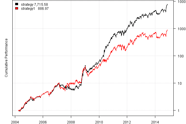

plot of chunk plot-5

	print(plotbt.strategy.sidebyside(models, make.plot=F, return.table=T))

	strategy	strategy1
Period	Mar2004 - Nov2014	Mar2004 - Nov2014
Cagr	131.66	89.09
Sharpe	1.8	1.43
DVR	1.15	1.06
Volatility	55.29	55.41
MaxDD	-45.64	-56.77
AvgDD	-6.6	-6.91
VaR	-5.71	-5.76
CVaR	-8.11	-8.38
Exposure	99.96	99.93

Next, sensetivity analysis:

	models = list()
	
	sma.lens = 2:21
	vol.lens = 2:21

	
if(F) {
tic(10)	
	#*****************************************************************
	# Sensitivity Analysis
	#******************************************************************	
	for(n.vol in vol.lens) {
	  	spyVol = runSD(spyRets, n=n.vol)
		SPY.VOL = spyVol*100*sqrt(252)

		for(n.sma in sma.lens) {
  			SMA.VOL = SMA(prices$VXMT - SPY.VOL, n=n.sma)
  			signal = SMA.VOL > 0
    	
			data$weight[] = NA
				data$weight$XIV = iif(signal, 1, 0)
		    	data$weight$VXX = iif(signal, 0, 1)
			models[[ paste(n.sma, n.vol) ]] = bt.run.share(data, clean.signal=F, silent=T)
    	}
    }
toc(10)
}

tic(11)	
	#*****************************************************************
	# Sensitivity Analysis Cluster
	#******************************************************************
	run.backtest <- function(n.vol) {
		models = list()
	  	spyVol = runSD(spyRets, n=n.vol)
		SPY.VOL = spyVol*100*sqrt(252)

		for(n.sma in sma.lens) {
  			SMA.VOL = SMA(data$prices$VXMT - SPY.VOL, n=n.sma)
  			signal = SMA.VOL > 0
    	
			data$weight[] = NA
				data$weight$XIV = iif(signal, 1, 0)
		    	data$weight$VXX = iif(signal, 0, 1)
			models[[ paste(n.sma, n.vol) ]] = bt.run.share(data, clean.signal=F, silent=T)
    	}
    	
		# serialize and compress first
		models
	}
	
	#*****************************************************************
	# Run Cluster
	#*****************************************************************							
	load.packages('parallel')
		
	cl = setup.cluster(varlist='spyRets,sma.lens,data,run.backtest',envir=environment())
		
	out = clusterApplyLB(cl, vol.lens, function(j) { run.backtest(j) } )	

	stopCluster(cl)	
	
	models = do.call(c, out)
	
toc(11)

Elapsed time is 18.29 seconds

	#*****************************************************************
	# Create Report
	#******************************************************************
	out = plotbt.strategy.sidebyside(models, return.table=T, make.plot = F)
	
	# allocate matrix to store backtest results
	dummy = matrix('', len(vol.lens), len(sma.lens))
	    colnames(dummy) = paste('S', sma.lens)
	    rownames(dummy) = paste('V', vol.lens)
	     
	names = spl('Sharpe,Cagr,DVR,MaxDD')
	 
	for(i in names) {
	    dummy[] = ''
	     
	    for(n.vol in vol.lens)
	    	for(n.sma in sma.lens)	        
	            dummy[ paste('V', n.vol), paste('S', n.sma)] =
	                out[i, paste(n.sma, n.vol) ]
	             
		print(i, ':')
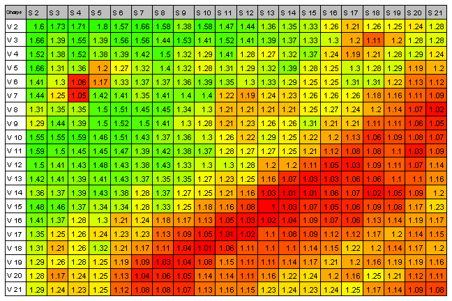
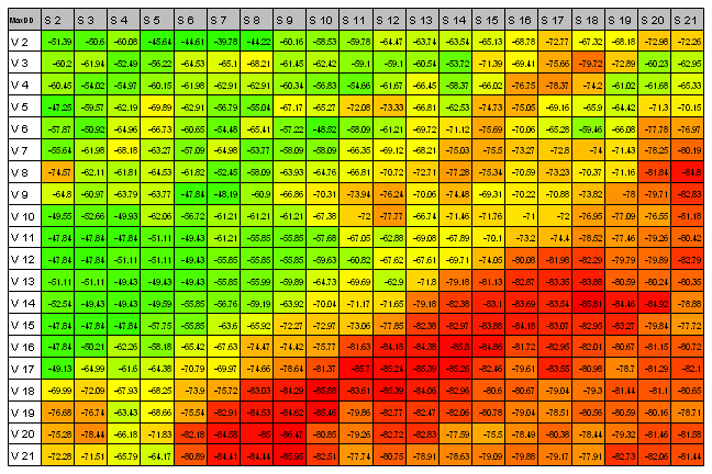
	    plot.table(dummy, smain = i, highlight = T, colorbar = F)
	 
	}

Sharpe :

plot of chunk plot-8

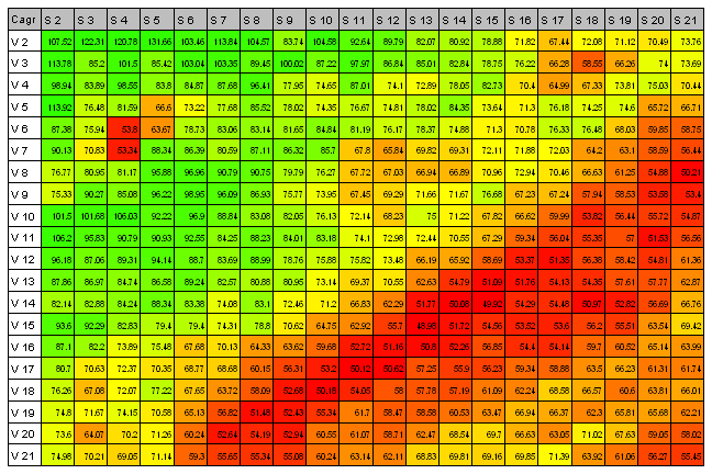
Cagr :

plot of chunk plot-8

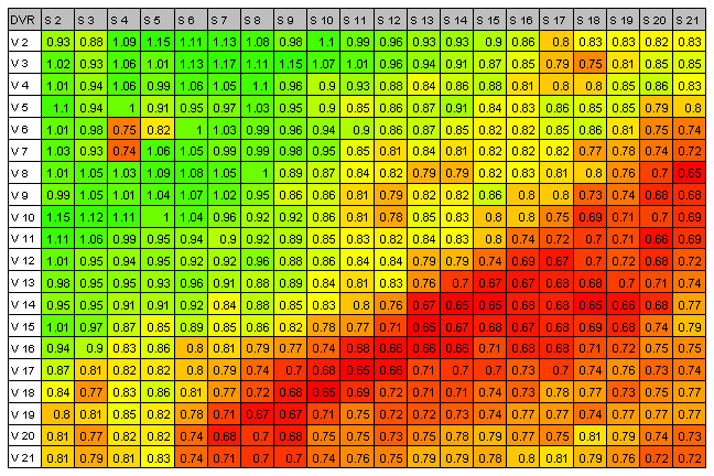
DVR :

plot of chunk plot-8

MaxDD :

plot of chunk plot-8

	load.packages('ggplot2,reshape2')
	plot.data = melt(dummy)
		colnames(plot.data) = c("vol", "sma", "Sharpe")
	
	plot.data$SMA = as.numeric(gsub("S", "", plot.data$sma))
	plot.data$VOL = as.numeric(gsub("V", "", plot.data$vol))
	plot.data$Sharpe = scale(as.numeric(plot.data$Sharpe))

	ggplot(plot.data, aes(x=SMA, y=VOL, fill=Sharpe))+
		geom_tile()+	
		scale_fill_gradient2(high="skyblue", mid="blue", low="red")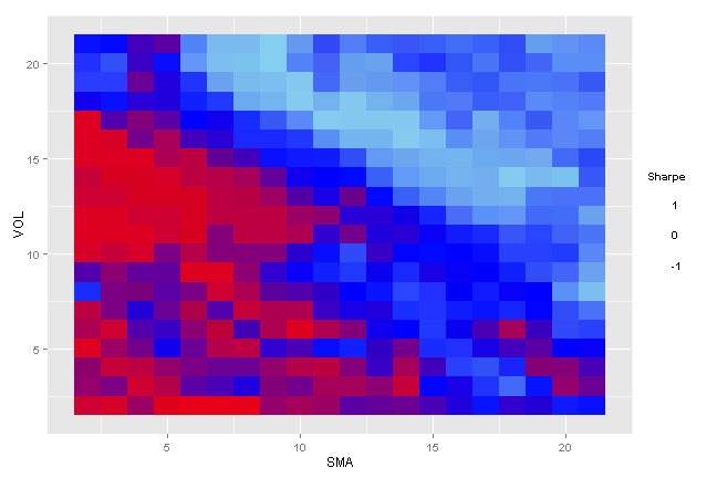

plot of chunk plot-8

Helmuth Vollmeier says my app The strategy employs a SINGLE variable (the SMA of a ratio of 2 points on the term structure). The strategy is robust over the whole range. Even if you want there is almost no way to get a mediocre performance ! No clever optimization will change this fact. To ‘harvest’ the premium I think the simplest strategies are the most efficient,

A side note concerning the entry : an entry on the NEXT close is even more profitable than entering on the close ( there is some short term mean-reversion)

90 days sma

vxx xiv ratio ma action ret

2014-11-13 0.0103 -0.0128 0.8942 0.9162 -1 -0.0128 2014-11-14 0.0032 -0.0024 0.9002 0.9162 -1 -0.0024 2014-11-17 -0.0021 0.0024 0.8949 0.9162 -1 0.0024 2014-11-18 -0.0175 0.0167 0.89 0.9162 -1 0.0167 2014-11-19 0.0242 -0.0244 0.8917 0.9161 -1 -0.0244 2014-11-20 -0.0104 0.0101 0.8939 0.9163 -1 0.0101

delta (term structure slope) = VIX - VXV

	load.packages('quantmod')
	tickers = spl('VIX=^VIX,VXV=^VXV,VXX+VXX.LONG,XIV+XIV.LONG')
	
	raw.data <- new.env()
    raw.data$VXX.LONG = make.stock.xts(read.xts("data/VXXlong.TXT", format='%Y-%m-%d'))

    raw.data$XIV.LONG = make.stock.xts(read.xts("data/XIVlong.TXT", format='%Y-%m-%d'))

    
	data <- new.env()
	getSymbols.extra(tickers, src = 'yahoo', from = '1970-01-01', env = data, raw.data = raw.data, auto.assign = T)
		for(i in ls(data)) data[[i]] = adjustOHLC(data[[i]], use.Adjusted=T)
		
#	data.CBOE = load.VXX.CBOE()
#		futures  = extract.VXX.CBOE(data.CBOE, 'Settle', 1:7)
#	data$ratio = make.xts(futures[,2]/futures[,5],data.CBOE$dates)
#		data$ratio[1:max(which(is.na(data$ratio)))] = NA
	
	bt.prep(data, align='remove.na')
  
	bt.start.dates(data)

Start        XIV "2006-07-17" VIX "2006-07-17" VXV "2006-07-17" VXX "2006-07-17"

	prices = data$prices
	ret = prices / mlag(prices) - 1
	
	#last(round(cbind(ret$VXX, ret$XIV, data$ratio),4),6)	
	#last(round(cbind(ret$VXX, ret$XIV, prices$VIX / prices$VXV),4),7)
	
	
data$ratio = prices$VIX / prices$VXV	
	
	sma = SMA(data$ratio, 90)
		
	signal = iif(data$ratio > sma, iif(data$ratio > 1, 1, 0), iif(data$ratio < 1, -1, 0))
	
#	write.xts(cbind(prices$VXX / mlag(prices$VXX) - 1,
#		prices$XIV / mlag(prices$XIV) - 1,
#		data$ratio,	sma, signal), '1.csv')
	


	
	
	#*****************************************************************
	# Code Strategies
	#*****************************************************************
	models = list()

	data$weight[] = NA
    	data$weight$VXX = iif(signal == 1, 1, 0)	
		data$weight$XIV = iif(signal == -1, 1, 0)
	models$strategy = bt.run.share(data, clean.signal=F, silent=T)
	
	data$weight[] = NA
    	data$weight$VXX = iif(signal == 1, 1, 0)	
		data$weight$XIV = iif(signal == -1, 1, 0)
	models$strategy1 = bt.run.share(data, do.lag=2, clean.signal=F, silent=T)

	#*****************************************************************
	# Create Report
	#*****************************************************************
	plotbt(models, plotX = T, log = 'y', LeftMargin = 3, main = NULL)
		mtext('Cumulative Performance', side = 2, line = 1)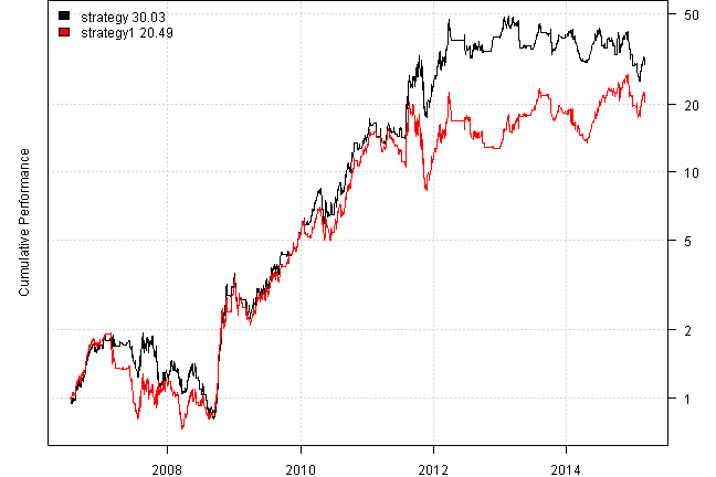

plot of chunk plot-9

	print(plotbt.strategy.sidebyside(models, make.plot=F, return.table=T))

	strategy	strategy1
Period	Jul2006 - Mar2015	Jul2006 - Mar2015
Cagr	48.16	41.76
Sharpe	1.05	0.96
DVR	0.87	0.85
Volatility	49.17	49.27
MaxDD	-58.71	-62.21
AvgDD	-8.61	-9.11
VaR	-5.1	-4.96
CVaR	-7.75	-7.63
Exposure	68.92	68.92

Investigate:

http://www.godotfinance.com/pdf/DynamicVIXFuturesVersion2Rev1.pdf
http://www.godotfinance.com/workingpapers/

Good way to use this high performance strategy in your portfolio is to balance it with other positions. For example, please see Barbell investing with XIV / SVXY at Don’t Fear the Bear blog

(this report was produced on: 2015-03-12)

Systematic Investor's Blog About Contact

Volatility Strategy from TradingTheOdds

Related Posts

RFinance 2016 15 May 2016

Benchmark Plus 14 Apr 2016

Exponentially Weighted Volatility using RCPP 10 Apr 2016