Synthetic Volatility Index
03 Feb 2015To install Systematic Investor Toolbox (SIT) please visit About page.
There is an interesting series of articles about Synthetic Volatility Index at QuantLab
- Synthetic Volatility Index Quantified Part 3
- Engineering a Synthetic Volatility Index Part 2
- Engineering a Synthetic Volatility Index Part 1
The objective set by QuantLab is to create Synthetic Volatility Index that 1) when applied to the S&P 500 mirrors the VIX index as closely as possible and 2) relies solely on price as an input so that it can be applied to any market index
The solution outlined is the Synthetic Volatility Index: > Mov(ATR(1)/C,20,S)
Below I will try to adapt a code from the posts:
#*****************************************************************
# Load historical data
#*****************************************************************
library(SIT)
load.packages('quantmod')

tickers = 'SP=^GSPC,VIX=^VIX'

data <- new.env()
getSymbols.extra(tickers, src = 'yahoo', from = '1970-01-01', env = data, auto.assign = T)
for(i in ls(data)) data[[i]] = adjustOHLC(data[[i]], use.Adjusted=T)
bt.prep(data, align='remove.na', fill.gaps = T)

#*****************************************************************
# Plot daya
#*****************************************************************
layout(1:3)
plota(data$SP, type='l', plotX=F)
	plota.legend('SP','black',data$SP)

plota(data$VIX, type='l', plotX=F)
	plota.legend('VIX','black',data$VIX)

vix.proxy = SMA( ATR(HLC(data$SP),1)[,"atr"] / Cl(data$SP), 20 )
cor.vix = cor(vix.proxy, Cl(data$VIX), use='complete.obs',method='pearson')
plota(vix.proxy, type='l', main=paste('Correlation with VIX:', to.percent(cor.vix)))
	plota.legend('ATR 20','black',vix.proxy)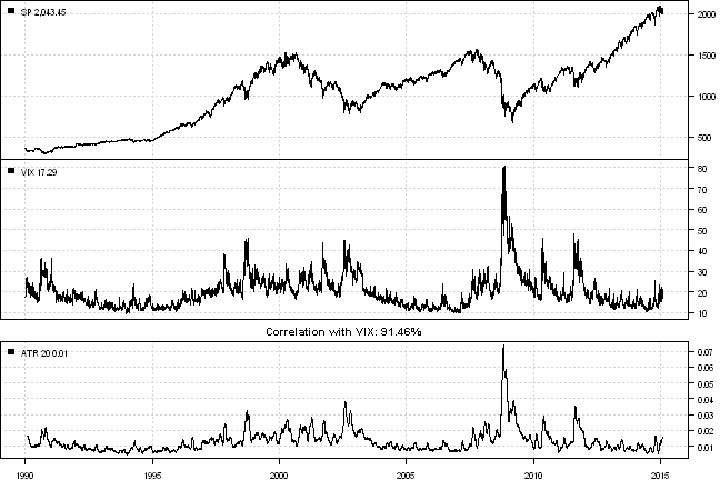
layout(1)
temp = as.xts(list(VIX = Cl(data$VIX), Vix.Proxy = vix.proxy))
plota.matplot(scale.one(na.omit(temp)))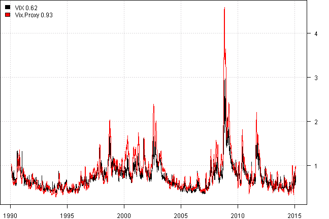
#*****************************************************************
# Test strategy
#*****************************************************************
vol.proxy = SMA( ATR(HLC(data$SP),1)[,"atr"] / Cl(data$SP), 20 )
high.vol.regime = vol.proxy > SMA(vol.proxy, 40)
low.vol.regime = vol.proxy < SMA(vol.proxy, 40)

layout(1:2)
index = '2013:10::'

highlight = high.vol.regime[index]

plota(data$SP[index], type='l', plotX=F, x.highlight = highlight)
  plota.legend('SP,HIGH VOL','black,orange')
plota(vol.proxy[index], type='l', x.highlight = highlight)
  plota.lines(SMA(vol.proxy, 40), col='blue')
  plota.legend('SP VOL PROXY, 40SMA','black,blue')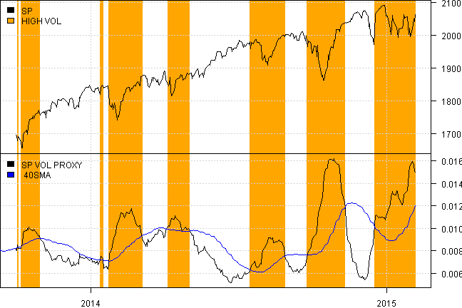
#*****************************************************************
# Test strategy
#*****************************************************************
models = list()

data$weight[] = NA
	data$weight$SP = 1
models$SP = bt.run.share(data, clean.signal=T, silent=T)

data$weight[] = NA
	data$weight$SP = iif(low.vol.regime, 1, 0)
models$low.vol = bt.run.share(data, clean.signal=T, silent=T)

#*****************************************************************
# Report
#*****************************************************************
#strategy.performance.snapshoot(models, T)
layout(1)
plotbt(models, plotX = T, log = 'y', LeftMargin = 3, main = NULL)
	mtext('Cumulative Performance', side = 2, line = 1)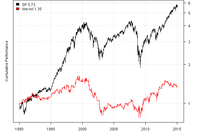
print(plotbt.strategy.sidebyside(models, make.plot=F, return.table=T))| SP | low.vol | |
|---|---|---|
| Period | Jan1990 - Feb2015 | Jan1990 - Feb2015 |
| Cagr | 7.2 | 1.21 |
| Sharpe | 0.47 | 0.16 |
| DVR | 0.34 | 0 |
| Volatility | 18.11 | 11.51 |
| MaxDD | -56.78 | -52.86 |
| AvgDD | -2.5 | -3.79 |
| VaR | -1.74 | -1.11 |
| CVaR | -2.69 | -1.89 |
| Exposure | 99.98 | 51.91 |
The estimate is similar to other volatility estimates available from TTR package:
ohlc = OHLC(data$SP)
temp = as.xts(list(
  VIX = Cl(data$VIX),
  Vix.Proxy = vix.proxy,
  Vol.Close = volatility(ohlc, n=20, calc='close'),
  Vol.GK = volatility(ohlc, n=20, calc='garman'),
  Vol.Parkinson = volatility(ohlc, n=20, calc='parkinson'),
  Vol.RS = volatility(ohlc, n=20, calc='rogers')
))

print(to.percent(cor(temp, use='complete.obs',method='pearson'),0))| VIX | Vix.Proxy | Vol.Close | Vol.GK | Vol.Parkinson | Vol.RS | |
|---|---|---|---|---|---|---|
| VIX | 100% | 91% | 89% | 91% | 91% | 90% |
| Vix.Proxy | 91% | 100% | 98% | 99% | 100% | 98% |
| Vol.Close | 89% | 98% | 100% | 96% | 98% | 93% |
| Vol.GK | 91% | 99% | 96% | 100% | 99% | 100% |
| Vol.Parkinson | 91% | 100% | 98% | 99% | 100% | 98% |
| Vol.RS | 90% | 98% | 93% | 100% | 98% | 100% |
(this report was produced on: 2015-02-06)