Stock Bond Model from Don't Fear the Bear
13 Dec 2014To install Systematic Investor Toolbox (SIT) please visit About page.
Another interesing post from Don’t Fear the Bear : A stock bond model based on the average investor allocation to equities that is based on the The Single Greatest Predictor of Future Stock Market Returns
The main indicator:
Investor Allocation to Stocks (Average) = Market Value of All Stocks / (Market Value of All Stocks + Total Liabilities of All Real Economic Borrowers)
is constructed using FRED data in the here
It is based on the following data:
- (a) Nonfinancial corporate business; corporate equities; liability, Level, Millions of Dollars, Not Seasonally Adjusted (NCBEILQ027S)
- (b) Nonfinancial Corporate Business; Credit Market Instruments; Liability, Billions of Dollars, Seasonally Adjusted (BCNSDODNS)
- (c) Households and Nonprofit Organizations; Credit Market Instruments; Liability, Level, Billions of Dollars, Seasonally Adjusted (CMDEBT)
- (d) Federal Government; Credit Market Instruments; Liability, Level, Billions of Dollars, Seasonally Adjusted (FGSDODNS)
- (e) State and Local Governments, Excluding Employee Retirement Funds; Credit Market Instruments; Liability, Level, Billions of Dollars, Seasonally Adjusted (SLGSDODNS)
- (f) Financial business; corporate equities; liability, Level, Millions of Dollars, Not Seasonally Adjusted (FBCELLQ027S)
- (g) Rest of the World; Credit Market Instruments; Liability, Level, Billions of Dollars, Seasonally Adjusted (DODFFSWCMI)
Please not the that (a) and (f) are Millions, rest in Billions; hence there is division by 1000 in the formula below:
Investor Allocation to Stocks (Average) = ((a+f)/1000)/(((a+f)/1000)+b+c+d+e+g)
Load historical data from FRED:
#*****************************************************************
# Load historical data
#*****************************************************************
library(SIT)
load.packages('quantmod')
tickers = spl('A=NCBEILQ027S,B=BCNSDODNS,C=CMDEBT,D=FGSDODNS,E=SLGSDODNS,F=FBCELLQ027S,G=DODFFSWCMI')

metric.data <- new.env()
getSymbols.extra(tickers, src = 'FRED', from = '1900-01-01', env = metric.data, auto.assign = T, getSymbols.fn=quantmod:::getSymbols)
Next let’s compute the Stock Allocation:
metric.data$StockAllocation = with(metric.data, ((A+F)/1000)/(((A+F)/1000)+B+C+D+E+G))

metric.data$AverageRatio  = SMA(ifna.prev(metric.data$StockAllocation),4)

metric.data$RelativeAverageRatio = 1 - (metric.data$AverageRatio - 0.25) / 0.20
  metric.data$RelativeAverageRatio = iif(metric.data$RelativeAverageRatio > 1, 1, metric.data$RelativeAverageRatio)
  metric.data$RelativeAverageRatio = iif(metric.data$RelativeAverageRatio < 0, 0, metric.data$RelativeAverageRatio)
  colnames(metric.data$RelativeAverageRatio) = 'RelativeAverageRatio'

plota(metric.data$RelativeAverageRatio, type='l')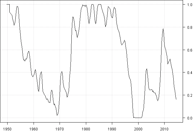
print(last(metric.data$RelativeAverageRatio, 20))| RelativeAverageRatio | |
|---|---|
| 2009-10-01 | 0.7386075 |
| 2010-01-01 | 0.6448204 |
| 2010-04-01 | 0.6192706 |
| 2010-07-01 | 0.6073752 |
| 2010-10-01 | 0.5777071 |
| 2011-01-01 | 0.5408631 |
| 2011-04-01 | 0.4747850 |
| 2011-07-01 | 0.4852374 |
| 2011-10-01 | 0.4993816 |
| 2012-01-01 | 0.5045022 |
| 2012-04-01 | 0.5189942 |
| 2012-07-01 | 0.4680151 |
| 2012-10-01 | 0.4474356 |
| 2013-01-01 | 0.4258632 |
| 2013-04-01 | 0.3850559 |
| 2013-07-01 | 0.3436522 |
| 2013-10-01 | 0.2763624 |
| 2014-01-01 | 0.2348901 |
| 2014-04-01 | 0.1889742 |
| 2014-07-01 | 0.1637294 |
Now let’s test the strategy with Vanguard funds:
#*****************************************************************
# Test Strategy
#*****************************************************************
tickers='STOCK=VFINX,BOND=VUSTX'

data <- new.env()
getSymbols.extra(tickers, src = 'yahoo', from = '1970-01-01', env = data, auto.assign = T)
for(i in ls(data)) data[[i]] = adjustOHLC(data[[i]], use.Adjusted=T)

print(bt.start.dates(data))| Start | |
|---|---|
| STOCK | 1987-03-27 |
| BOND | 1989-12-14 |
data$StockAllocation = make.stock.xts(metric.data$RelativeAverageRatio)

bt.prep(data, align='keep.all')

prices = data$prices

prices$StockAllocation = ifna.prev(prices$StockAllocation)

models = list()


#*****************************************************************
# Code Strategies
#*****************************************************************

data$weight[] = NA
	data$weight$BOND = 1
models$BOND = bt.run.share(data, clean.signal=F, silent=T)

data$weight[] = NA
	data$weight$STOCK = 1
models$STOCK = bt.run.share(data, clean.signal=F, silent=T)

data$weight[] = NA
	data$weight$STOCK = prices$StockAllocation
  data$weight$BOND  = 1 - prices$StockAllocation
models$strategy = bt.run.share(data, clean.signal=F, silent=T)


models = bt.trim(models, dates = '1990::')


#*****************************************************************
# Create Report
#*****************************************************************
plotbt(models, plotX = T, log = 'y', LeftMargin = 3, main = NULL)
mtext('Cumulative Performance', side = 2, line = 1)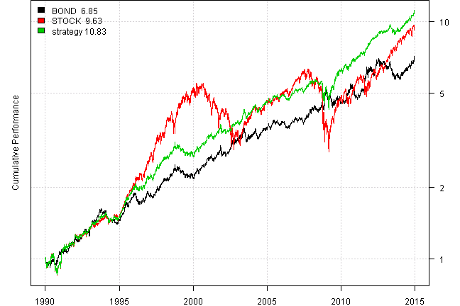
print(plotbt.strategy.sidebyside(models, make.plot=F, return.table=T))| BOND | STOCK | strategy | |
|---|---|---|---|
| Period | Jan1990 - Dec2014 | Jan1990 - Dec2014 | Jan1990 - Dec2014 |
| Cagr | 8 | 9.49 | 10 |
| Sharpe | 0.78 | 0.59 | 1.02 |
| DVR | 0.74 | 0.48 | 0.94 |
| Volatility | 10.45 | 18.06 | 9.71 |
| MaxDD | -18.78 | -55.25 | -25.07 |
| AvgDD | -2.16 | -2.22 | -1.38 |
| VaR | -1.05 | -1.73 | -0.9 |
| CVaR | -1.45 | -2.67 | -1.41 |
| Exposure | 100 | 100 | 100 |
There is more to investigate. The fun part is that i was able to replicate this strategy in about 2 hours.
(this report was produced on: 2014-12-25)