Simulating correlated random walks with Copulas
16 Jan 2015To install Systematic Investor Toolbox (SIT) please visit About page.
Another great article from mktstk: Simulating correlated random walks with Copulas
We can replicate this example using R
	#*****************************************************************
	# Load historical data
	#******************************************************************
	library(SIT)
	load.packages('quantmod')

filename = 'intraday.Rdata'
if(!file.exists(filename)) {
	data <- new.env()
		data$YHOO = getSymbol.intraday.google('YHOO', 'NASDAQ', 60, '15d')
		data$FB = getSymbol.intraday.google('FB', 'NASDAQ', 60, '15d')
	bt.prep(data, align='remove.na')
save(data, file=filename)
}
load(file=filename)

	#*****************************************************************
	# Generate simulations
	#******************************************************************
	prices = data$prices
 	n = ncol(prices)
	rets = diff(log(prices))
		rets = coredata(na.omit(rets))

 # Plot prices
 matplot(exp(apply(rets,2,cumsum)), type='l', main='Actual Price path')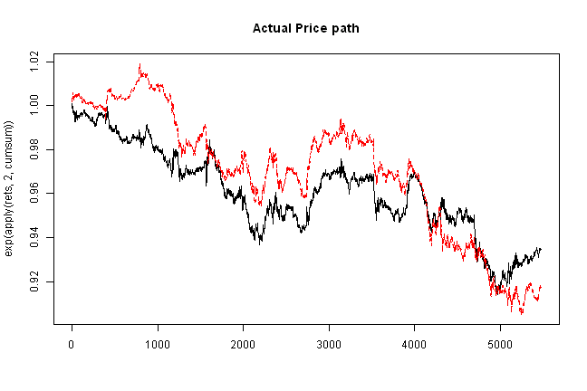
# helper function to visualize distribution
visualize.rets = function(fit.sim) {
labs = colnames(rets)
xhist = hist(fit.sim[,1], plot=FALSE)
yhist = hist(fit.sim[,2], plot=FALSE)
top =max(c(xhist$counts, yhist$counts))
layout(matrix(c(2,0,1,3),2,2,byrow=TRUE), c(3,1), c(1,3), TRUE)
par(mar=c(3,3,1,1))
plot(fit.sim[,1], fit.sim[,2], xlab=labs[1], ylab=labs[2], col='blue', las=1)
par(mar=c(0,3,1,1))
barplot(xhist$counts, axes=FALSE, ylim=c(0, top), space=0,col="light green")
barplot(yhist$counts, axes=FALSE, xlim=c(0, top), space=0, horiz=TRUE,col="light blue")
}
# Helper function to check Copula fit
copula.check = function(fit.sim) {
# plot simulated vs actual
labs = colnames(rets)
layout(1)
plot(rets[,1], rets[,2], xlab=labs[1], ylab=labs[2], col='blue', las=1)
points(fit.sim[,1], fit.sim[,2], col='red')
# compare stats for simulated vs actual
temp = matrix(0,nr=5,nc=2)
colnames(temp) = spl('Actual,Simulated')
rownames(temp) = c('Correlation', paste('Mean', labs), paste('StDev', labs))
temp[1,] = c(cor(rets)[1,2], cor(fit.sim)[1,2])
temp[2:3,] = 252 * cbind(apply(rets, 2, mean), apply(fit.sim, 2, mean))
temp[4:5,] = sqrt(252) * cbind(apply(rets, 2, sd), apply(fit.sim, 2, sd))
print(round(100*temp,2))
# check if returns come from same distributions
for (i in 1:2) {
print(labs[i])
print(ks.test(rets[,i], fit.sim[i]))
}
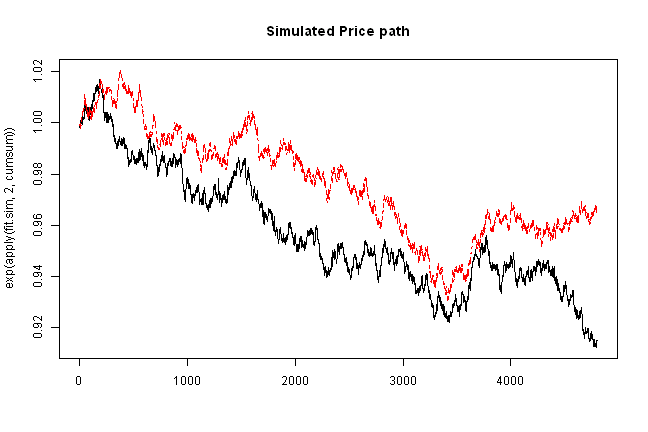
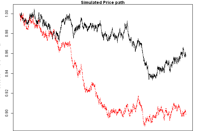
# plot simulated price path
matplot(exp(apply(fit.sim,2,cumsum)), type='l', main='Simulated Price path')
}
# fit Copula
load.packages('copula')package ‘gsl’ successfully unpacked and MD5 sums checked package ‘ADGofTest’ successfully unpacked and MD5 sums checked package ‘stabledist’ successfully unpacked and MD5 sums checked package ‘mvtnorm’ successfully unpacked and MD5 sums checked package ‘pspline’ successfully unpacked and MD5 sums checked package ‘copula’ successfully unpacked and MD5 sums checked
The downloaded binary packages are in C:\Temp\RtmpCw8dcM\downloaded_packages
 gumbel.cop = gumbelCopula(dim=n)
 	uniform.data = pobs(rets)
 gumbel = fitCopula(gumbel.cop, uniform.data, method="ml")

 # create custom distribution by combining fitted margins with fitted copula
 margins=c("norm","norm")
 paramMargins=apply(rets,2,function(x) list(mean=mean(x), sd=sd(x)))

 fit = mvdc(copula = gumbelCopula(gumbel@estimate, dim=n),
		margins=margins,paramMargins=paramMargins)

	# simulate from fitted distn
	fit.sim = rMvdc(4800, fit)

 copula.check(fit.sim)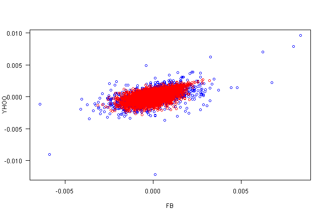
| Actual | Simulated | |
|---|---|---|
| Correlation | 57.13 | 57.38 |
| Mean FB | -0.31 | -0.47 |
| Mean YHOO | -0.40 | -0.17 |
| StDev FB | 1.24 | 1.25 |
| StDev YHOO | 1.23 | 1.23 |
FB
	Two-sample Kolmogorov-Smirnov test

data:  rets[, i] and fit.sim[i]
D = 0.9404, p-value = 0.3395
alternative hypothesis: two-sided
YHOO
	Two-sample Kolmogorov-Smirnov test

data:  rets[, i] and fit.sim[i]
D = 0.8792, p-value = 0.4222
alternative hypothesis: two-sided
visualize.rets(fit.sim)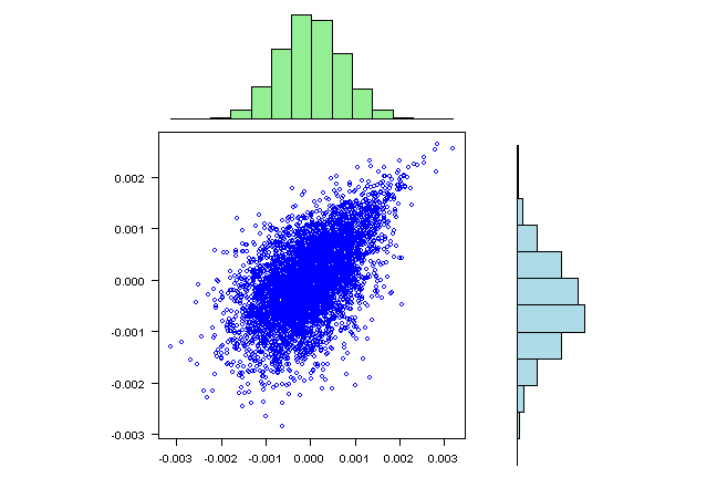
	# alternatively we can do it by hand, please note to go from uniform data
 # to original data, we can use quantile function
 # i.e [simulation by inverse cdf](https://xianblog.wordpress.com/2015/01/14/simulation-by-inverse-cdf/)
 # qnorm(runif(10^8)) and rnorm(10^8) are equivalent
	uniform.sim = rCopula(4800, gumbelCopula(gumbel@estimate, dim=n))
	fit.sim2 = cbind(
		qnorm(uniform.sim[,1],mean(rets[,1]),sd(rets[,1])),
		qnorm(uniform.sim[,2],mean(rets[,2]),sd(rets[,2]))
	)

 copula.check(fit.sim2)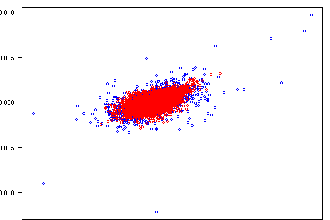
| Actual | Simulated | |
|---|---|---|
| Correlation | 57.13 | 57.14 |
| Mean FB | -0.31 | -0.22 |
| Mean YHOO | -0.40 | -0.56 |
| StDev FB | 1.24 | 1.24 |
| StDev YHOO | 1.23 | 1.21 |
FB
	Two-sample Kolmogorov-Smirnov test

data:  rets[, i] and fit.sim[i]
D = 0.7791, p-value = 0.5787
alternative hypothesis: two-sided
YHOO
	Two-sample Kolmogorov-Smirnov test

data:  rets[, i] and fit.sim[i]
D = 0.795, p-value = 0.5525
alternative hypothesis: two-sided
visualize.rets(fit.sim2)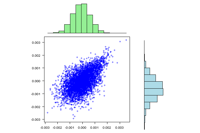
visualize.rets(rets)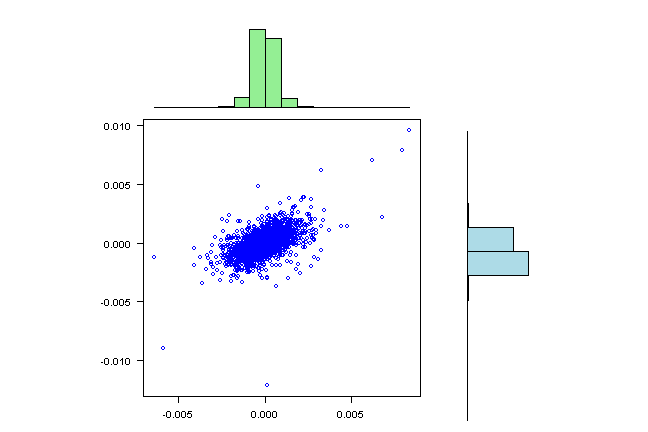
Please note that Standard Deviation is huge relative to the Mean, which is close to zero; hence, we are very likely to get positive and negative outcomes in some cases.
For additional references on the topic, I found following references very useful:
- Generating values from copula using copula package in R
- Simulating returns using copula and SPD distribution
- Info from Eric Zivot’s site
- R Code
- Principal Component Analysis (PCA) vs Ordinary Least Squares (OLS): A Visual Explanation
- Stochastic Simulation With Copulas in R
- Even Simpler Multivariate Correlated Simulations
-
Third, and Hopefully Final, Post on Correlated Random Normal Generation (Cholesky Edition)
- Ambhas
- simulation by inverse cdf > system.time(qnorm(runif(10^8))) > system.time(rnorm(10^8))
(this report was produced on: 2015-01-17)