Visualizing Price Scenarios
06 Jun 2015To install Systematic Investor Toolbox (SIT) please visit About page.
Newfound Research shared an interesting post: Volatility Through a Different Lens that features a chart of Sector Energy ETF(XLE) with historical price scenarios highlighted with various colors.
This reminded me of the post i wrote back in 2012: Classical Technical Patterns Below I will use same machinery to automatically find scenarios in historical price data.
#*****************************************************************
# Load historical data
#*****************************************************************
library(SIT)
load.packages('quantmod')

ticker = 'XLE'
data = env()

getSymbols.extra(ticker, src = 'yahoo', from = '1970-01-01', env = data,  set.symbolnames = T, auto.assign = T)
	for(i in data$symbolnames) data[[i]] = adjustOHLC(data[[i]], use.Adjusted=T)
bt.prep(data, align='remove.na', fill.gaps = T)


#*****************************************************************
# Find extrema
#*****************************************************************
sample = data$XLE['2014:06:30::2015:06:04']

load.packages('sm')

# find extrema
obj = find.extrema( Cl(sample) )
	mhat.extrema.loc = obj$mhat.extrema.loc
	extrema.dir = obj$extrema.dir

#*****************************************************************
# Map extrema to data
#*****************************************************************
x = Cl(sample)
n = len(x)
temp = c(1, mhat.extrema.loc, n)
loc =  mhat.extrema.loc
for(i in 2:(len(temp)-1)) {
	index = round(temp[i] - (temp[i] - temp[i-1]) / 2) : round(temp[i] + (temp[i+1] - temp[i]) / 2)
	loc[i-1] = index[1] - 1 + iif(extrema.dir[i-1] > 0, which.max(x[index]), which.min(x[index]))
}

# do not allow extrema at the boundaries
margin = min(10, round(n * 0.1))
loc = loc[ loc >= margin & loc <= (n-margin)]

print(index(sample[loc]))
2014-08-07 2014-08-29 2014-10-14 2014-11-21 2014-12-15 2014-12-23 2015-01-15 2015-02-17 2015-03-13 2015-04-29
#*****************************************************************
# Plot
#*****************************************************************
highlight = sample[,1] * NA
	highlight[loc] = len(loc):1
	highlight[1] = len(loc) + 1
	dates = highlight[!is.na(highlight)]
	highlight[] = ifna.prev(highlight)

plota(sample)
	col = col.add.alpha(highlight, 50)
plota.x.highlight(highlight, highlight != 0, col)
plota.lines(sample)
	plota.lines(sample[loc], type='p', col='green', lwd=1, pch=19)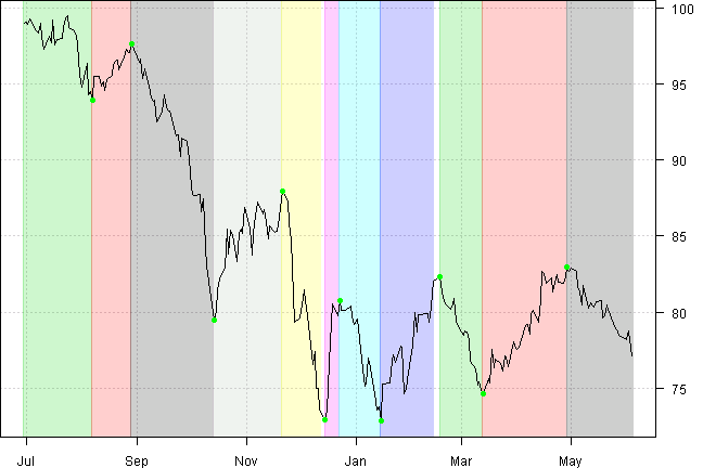
#*****************************************************************
# Compute Daily Average Log-Difference
#*****************************************************************
ret = diff(log(Cl(sample)))

stat = tapply(ret, highlight, mean, na.rm=T)

temp = data.frame(date = index(dates), col=as.vector(dates), stat = stat[match(dates, names(stat))])
	temp = na.omit(temp)

par(mar = c(6, 4, 2, 2))
barplot(temp$stat, col=col.add.alpha(temp$col, 50), names.arg=temp$date, las=2, main='Daily Average Log-Difference')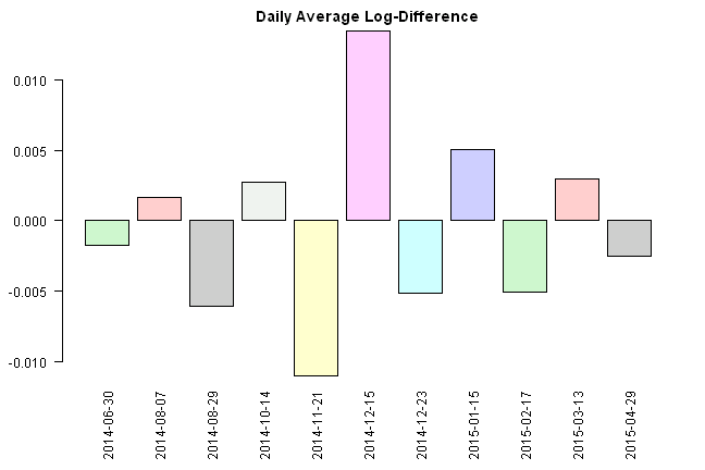
#*****************************************************************
# Compute Total Daily Log-Difference
#*****************************************************************
stat = tapply(ret, highlight, sum, na.rm=T)

temp = data.frame(date = index(dates), col=as.vector(dates), stat = stat[match(dates, names(stat))])
	temp = na.omit(temp)

par(mar = c(6, 4, 2, 2))
barplot(temp$stat, col=col.add.alpha(temp$col, 50), names.arg=temp$date, las=2, main='Total Daily Log-Difference')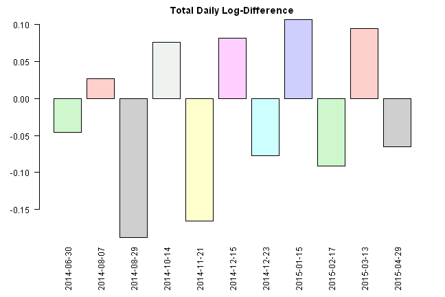
(this report was produced on: 2015-06-07)