Review of Momentum and Markowitz A Golden Combination paper
04 Jun 2015To install Systematic Investor Toolbox (SIT) please visit About page.
The Momentum and Markowitz: A Golden Combination (2015) by Keller, Butler, Kipnis paper is a review of practitioner’s tools to make mean variance optimization portfolio a viable solution. In particular, authors suggest and test:
- adding maximum weight limits and
- adding target volatility constraint
to control solution of mean variance optimization.
Below I will have a look at the results for the 8 asset universe:
- S&P 500
- EAFE
- Emerging Markets
- US Technology Sector
- Japanese Equities
- 10-Year Treasuries
- T-Bills
- High Yield Bonds
First, let’s load historical data for all assets
#*****************************************************************
# Load historical data
#*****************************************************************
library(SIT)
load.packages('quantmod')

# load saved Proxies Raw Data, data.proxy.raw
# please see http://systematicinvestor.github.io/Data-Proxy/ for more details
load('data/data.proxy.raw.Rdata')

N8.tickers = '
US.EQ = VTI + VTSMX + VFINX
EAFE = EFA + VDMIX + VGTSX
EMER.EQ = EEM + VEIEX
TECH.EQ = QQQ + ^NDX
JAPAN.EQ = EWJ + FJPNX
MID.TR = IEF + VFITX
US.CASH = BIL + TB3M,
US.HY = HYG + VWEHX
'

data = env()
getSymbols.extra(N8.tickers, src = 'yahoo', from = '1970-01-01', env = data, raw.data = data.proxy.raw, set.symbolnames = T, auto.assign = T)
	for(i in data$symbolnames) data[[i]] = adjustOHLC(data[[i]], use.Adjusted=T)
bt.prep(data, align='remove.na', fill.gaps = T)
Next, let’s test the functionality of kellerCLAfun from Appendix A
#*****************************************************************
# Run tests, monthly data - works
#*****************************************************************
data = bt.change.periodicity(data, periodicity = 'months')

plota.matplot(scale.one(data$prices))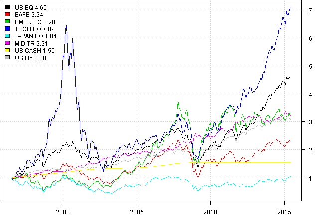
prices = data$prices

res = kellerCLAfun(prices, returnWeights = T, 0.25, 0.1, c('US.CASH', 'MID.TR'))

plotbt.transition.map(res[[1]]['2013::'])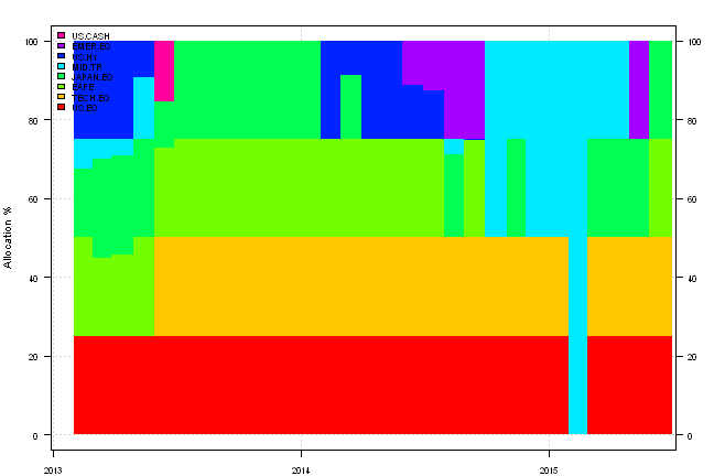
plota(cumprod(1 + res[[2]]), type='l')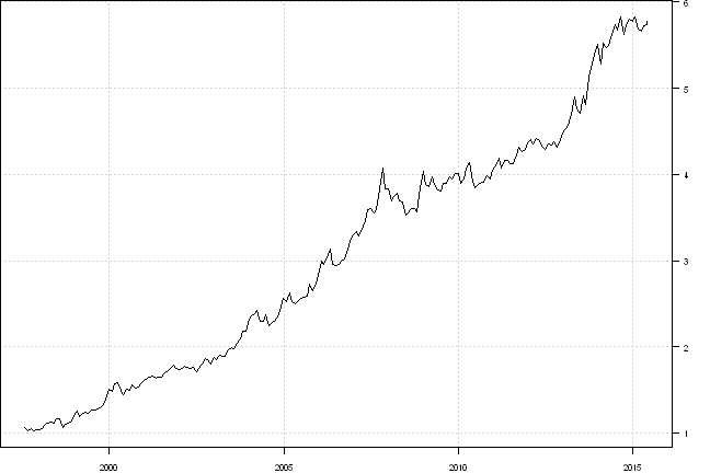
Next, let’s create a benchmark and set up commision structure to be used for all tests.
#*****************************************************************
# Create a benchmark
#*****************************************************************
models = list()

commission = list(cps = 0.01, fixed = 10.0, percentage = 0.0)

data$weight[] = NA
	data$weight$US.EQ = 1
	data$weight[1:12,] = NA
models$US.EQ = bt.run.share(data, clean.signal=T, commission=commission, trade.summary=T, silent=T)
Next, let’s take weights from the kellerCLAfun and use them to create a back-test
#*****************************************************************
# transform kellerCLAfun into model results
#*****************************************************************
#models$CLA = list(weight = res[[1]], ret = res[[2]], equity = cumprod(1 + res[[2]]), type = "weight")

obj = list(weights = list(CLA = res[[1]]), period.ends = index(res[[1]]))
models = c(models, create.strategies(obj, data, commission=commission, trade.summary=T, silent=T)$models)
We can easily replicate same results with base SIT functionality
#*****************************************************************
# Replicate using base SIT functionality
#*****************************************************************
weight.limit = data.frame(last(prices))
	weight.limit[] = 0.25
	weight.limit$US.CASH = weight.limit$MID.TR = 1

obj = portfolio.allocation.helper(data$prices,
	periodicity = 'months', lookback.len = 12, silent=T,
		const.ub = weight.limit,
		create.ia.fn = 	function(hist.returns, index, nperiod) {
			ia = create.ia(hist.returns, index, nperiod)
			ia$expected.return = (last(hist.returns,1) + colSums(last(hist.returns,3)) +
				colSums(last(hist.returns,6)) + colSums(last(hist.returns,12))) / 22
			ia
		},
		min.risk.fns = list(
			TRISK = target.risk.portfolio(target.risk = 0.1, annual.factor=12)
		)
	)

models = c(models, create.strategies(obj, data, commission=commission, trade.summary=T, silent=T)$models)
Another idea is to use Pierre Chretien’s Averaged Input Assumptions
#*****************************************************************
# Let's use Pierre's Averaged Input Assumptions
#*****************************************************************
obj = portfolio.allocation.helper(data$prices,
	periodicity = 'months', lookback.len = 12, silent=T,
		const.ub = weight.limit,
		create.ia.fn = 	create.ia.averaged(c(1,3,6,12), 0),
		min.risk.fns = list(
			TRISK.AVG = target.risk.portfolio(target.risk = 0.1, annual.factor=12)
		)
	)

models = c(models, create.strategies(obj, data, commission=commission, trade.summary=T, silent=T)$models)
Finally we are ready to look at the results
#*****************************************************************
# Plot back-test
#*****************************************************************
models = bt.trim(models)
#strategy.performance.snapshoot(models, T)
plotbt(models, plotX = T, log = 'y', LeftMargin = 3, main = NULL)
	mtext('Cumulative Performance', side = 2, line = 1)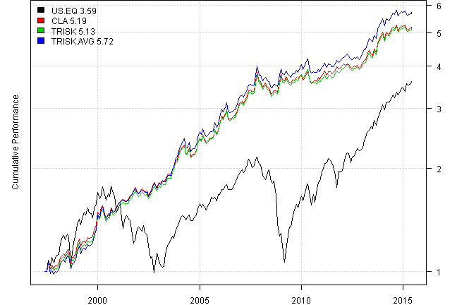
print(plotbt.strategy.sidebyside(models, make.plot=F, return.table=T, perfromance.fn=engineering.returns.kpi)) | US.EQ | CLA | TRISK | TRISK.AVG | |
|---|---|---|---|---|
| Period | May1997 - Jun2015 | May1997 - Jun2015 | May1997 - Jun2015 | May1997 - Jun2015 |
| Cagr | 7.36 | 9.57 | 9.49 | 10.16 |
| Sharpe | 0.53 | 1.02 | 1.01 | 1.04 |
| DVR | 0.33 | 1 | 0.98 | 1.01 |
| R2 | 0.63 | 0.98 | 0.97 | 0.97 |
| Volatility | 15.84 | 9.32 | 9.42 | 9.72 |
| MaxDD | -50.84 | -13.65 | -13.65 | -13.65 |
| Exposure | 99.08 | 99.08 | 99.08 | 99.08 |
| Win.Percent | 100 | 64.57 | 59.85 | 59.28 |
| Avg.Trade | 259.48 | 0.26 | 0.18 | 0.19 |
| Profit.Factor | NaN | 1.93 | 1.87 | 1.93 |
| Num.Trades | 1 | 717 | 1066 | 1051 |
layout(1)
barplot.with.labels(sapply(models, compute.turnover, data), 'Average Annual Portfolio Turnover') 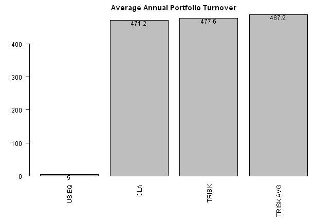
Our replication results are almost identical results to the results using kellerCLAfun.
Using Averaged Input Assumptions produces slightly better results.
I guess the main point that a reader should remember from reading Momentum and Markowitz: A Golden Combination (2015) by Keller, Butler, Kipnis paper is that it is a bad idea to blindly use the optimizer. Instead, you should apply common sense heuristics mentioned in the paper to make solution robust across time and various universes.
Supporting functions:
#*****************************************************************
# Appendix B. CLA code (in R) by Ilya Kipnis (QuantStratTradeR10) SSRN-id2606884.pdf
#*****************************************************************
require(quantmod)
require(PerformanceAnalytics)
require(TTR)

CCLA <- function(covMat, retForecast, maxIter = 1000,
	verbose = FALSE, scale = 252,
	weightLimit = .7, volThresh = .1)
{
	if(length(retForecast) > length(unique(retForecast))) {
		sequentialNoise <- seq(1:length(retForecast)) * 1e-12
		retForecast <- retForecast + sequentialNoise
	}

	#initialize original out/in/up status
	if(length(weightLimit) == 1) {
		weightLimit <- rep(weightLimit, ncol(covMat))
	}

	# sort return forecasts
	rankForecast <- length(retForecast) - rank(retForecast) + 1
	remainingWeight <- 1 #have 100% of weight to allocate
	upStatus <- inStatus <- rep(0, ncol(covMat))
	i <- 1

	# find max return portfolio
	while(remainingWeight > 0) {
		securityLimit <- weightLimit[rankForecast == i]
		if(securityLimit < remainingWeight) {
			upStatus[rankForecast == i] <- 1 #if we can't invest all remaining weight into the security
			remainingWeight <- remainingWeight - securityLimit
		} else {
			inStatus[rankForecast == i] <- 1
			remainingWeight <- 0
		}
		i <- i + 1
	}

	#initial matrices (W, H, K, identity, negative identity)
	covMat <- as.matrix(covMat)
	retForecast <- as.numeric(retForecast)
	init_W <- cbind(2*covMat, rep(-1, ncol(covMat)))
	init_W <- rbind(init_W, c(rep(1, ncol(covMat)), 0))
	H_vec <- c(rep(0, ncol(covMat)), 1)
	K_vec <- c(retForecast, 0)
	negIdentity <- -1*diag(ncol(init_W))
	identity <- diag(ncol(init_W))
	matrixDim <- nrow(init_W)
	weightLimMat <- matrix(rep(weightLimit, matrixDim), ncol=ncol(covMat), byrow=TRUE)
	#out status is simply what isn't in or up
	outStatus <- 1 - inStatus - upStatus

	#initialize expected volatility/count/turning points data structure
	expVol <- Inf
	lambda <- 100
	count <- 0
	turningPoints <- list()

	while(lambda > 0 & count < maxIter) {
		#old lambda and old expected volatility for use with numerical algorithms
		oldLambda <- lambda
		oldVol <- expVol
		count <- count + 1

		#compute W, A, B
		inMat <- matrix(rep(c(inStatus, 1), matrixDim), nrow = matrixDim, byrow = TRUE)
		upMat <- matrix(rep(c(upStatus, 0), matrixDim), nrow = matrixDim, byrow = TRUE)
		outMat <- matrix(rep(c(outStatus, 0), matrixDim), nrow = matrixDim, byrow = TRUE)
		W <- inMat * init_W + upMat * identity + outMat * negIdentity

		inv_W <- solve(W)
		modified_H <- H_vec - rowSums(weightLimMat* upMat[,-matrixDim] * init_W[,-matrixDim])
		A_vec <- inv_W %*% modified_H
		B_vec <- inv_W %*% K_vec

		#remove the last elements from A and B vectors
		truncA <- A_vec[-length(A_vec)]
		truncB <- B_vec[-length(B_vec)]

		#compute in Ratio (aka Ratio(1) in Kwan.xls)
		inRatio <- rep(0, ncol(covMat))
		inRatio[truncB > 0] <- -truncA[truncB > 0]/truncB[truncB > 0]

		#compute up Ratio (aka Ratio(2) in Kwan.xls)
		upRatio <- rep(0, ncol(covMat))
		upRatioIndices <- which(inStatus==TRUE & truncB < 0)

		if(length(upRatioIndices) > 0) {
			upRatio[upRatioIndices] <- (weightLimit[upRatioIndices] - truncA[upRatioIndices]) / truncB[upRatioIndices]
		}

		#find lambda -- max of up and in ratios
		maxInRatio <- max(inRatio)
		maxUpRatio <- max(upRatio)
		lambda <- max(maxInRatio, maxUpRatio)

		#compute new weights
		wts <- inStatus*(truncA + truncB * lambda) + upStatus * weightLimit + outStatus * 0

		#compute expected return and new expected volatility
		expRet <- t(retForecast) %*% wts
		expVol <- sqrt(wts %*% covMat %*% wts) * sqrt(scale)

		#create turning point data row and append it to turning points
		turningPoint <- cbind(count, expRet, lambda, expVol, t(wts))
		colnames(turningPoint) <- c("CP", "Exp. Ret.", "Lambda", "Exp. Vol.", colnames(covMat))
		turningPoints[[count]] <- turningPoint

		#binary search for volatility threshold -- if the first iteration is lower than the threshold,
		#then immediately return, otherwise perform the binary search until convergence of lambda
		if(oldVol == Inf & expVol < volThresh) {
			turningPoints <- do.call(rbind, turningPoints)
			threshWts <- tail(turningPoints, 1)
			return(list(turningPoints, threshWts))
		} else if(oldVol > volThresh & expVol < volThresh) {
			upLambda <- oldLambda
			dnLambda <- lambda
			meanLambda <- (upLambda + dnLambda)/2

			while(upLambda - dnLambda > .00001) {
				#compute mean lambda and recompute weights, expected return, and expected vol
				meanLambda <- (upLambda + dnLambda)/2
				wts <- inStatus*(truncA + truncB * meanLambda) + upStatus * weightLimit + outStatus * 0
				expRet <- t(retForecast) %*% wts
				expVol <- sqrt(wts %*% covMat %*% wts) * sqrt(scale)

				#if new expected vol is less than threshold, mean becomes lower bound
				#otherwise, it becomes the upper bound, and loop repeats
				if(expVol < volThresh) {
					dnLambda <- meanLambda
				} else {
					upLambda <- meanLambda
				}
			}

			#once the binary search completes, return those weights, and the corner points
			#computed until the binary search. The corner points aren't used anywhere, but they're there.
			threshWts <- cbind(count, expRet, meanLambda, expVol, t(wts))
			colnames(turningPoint) <- colnames(threshWts) <- c("CP", "Exp. Ret.", "Lambda", "Exp. Vol.", colnames(covMat))
			turningPoints[[count]] <- turningPoint
			turningPoints <- do.call(rbind, turningPoints)
			return(list(turningPoints, threshWts))
		}

		#this is only run for the corner points during which binary search doesn't take place
		#change status of security that has new lambda
		if(maxInRatio > maxUpRatio) {
			inStatus[inRatio == maxInRatio] <- 1 - inStatus[inRatio == maxInRatio]
			upStatus[inRatio == maxInRatio] <- 0
		} else {
			upStatus[upRatio == maxUpRatio] <- 1 - upStatus[upRatio == maxUpRatio]
			inStatus[upRatio == maxUpRatio] <- 0
		}
		outStatus <- 1 - inStatus - upStatus
	}


	#we only get here if the volatility threshold isn't reached
	#can actually happen if set sufficiently low
	turningPoints <- do.call(rbind, turningPoints)
	threshWts <- tail(turningPoints, 1)
	return(list(turningPoints, threshWts))
}


sumIsNa <- function(column) {
	return(sum(is.na(column)))
}

returnForecast <- function(prices) {
	forecast <- (ROC(prices, n = 1, type="discrete") + ROC(prices, n = 3, type="discrete") +
	ROC(prices, n = 6, type="discrete") + ROC(prices, n = 12, type="discrete"))/22
	forecast <- as.numeric(tail(forecast, 1))
	return(forecast)
}


kellerCLAfun <- function(prices, returnWeights = FALSE,
	weightLimit, volThresh, uncappedAssets)
{
	if(sum(colnames(prices) %in% uncappedAssets) == 0) {
		stop("No assets are uncapped.")
	}

	#initialize data structure to contain our weights
	weights <- list()
	#compute returns
	returns <- Return.calculate(prices)
	returns[1,] <- 0 #impute first month with zeroes
	ep <- endpoints(returns, on = "months")

	for(i in 2:(length(ep) - 12)) {
		priceSubset <- prices[ep[i]:ep[i+12]] #subset prices
		retSubset <- returns[ep[i]:ep[i+12]] #subset returns
		assetNAs <- apply(retSubset, 2, sumIsNa)
		zeroNAs <- which(assetNAs == 0)
		priceSubset <- priceSubset[, zeroNAs]
		retSubset <- retSubset[, zeroNAs]

		#remove perfectly correlated assets
		retCors <- cor(retSubset)
		diag(retCors) <- NA
		corMax <- round(apply(retCors, 2, max, na.rm = TRUE), 7)
		while(max(corMax) == 1) {
			ones <- which(corMax == 1)
			valid <- which(!names(corMax) %in% uncappedAssets)
			toRemove <- intersect(ones, valid)
			toRemove <- max(valid)
			retSubset <- retSubset[, -toRemove]
			priceSubset <- priceSubset[, -toRemove]
			retCors <- cor(retSubset)
			diag(retCors) <- NA
			corMax <- round(apply(retCors, 2, max, na.rm = TRUE), 7)
		}

		covMat <- cov(retSubset) #compute covariance matrix

		#Dr. Keller's return forecast
		retForecast <- returnForecast(priceSubset)
		uncappedIndex <- which(colnames(covMat) %in% uncappedAssets)
		weightLims <- rep(weightLimit, ncol(covMat))
		weightLims[uncappedIndex] <- 1

		cla <- CCLA(covMat = covMat, retForecast = retForecast, scale = 12,
			weightLimit = weightLims, volThresh = volThresh) #run CCLA algorithm
		CPs <- cla[[1]] #corner points
		wts <- cla[[2]] #binary search volatility targeting -- change this line and the next

		#if using max sharpe ratio golden search
		wts <- wts[, 5:ncol(wts)] #from 5th column to the end
		if(length(wts) == 1) {
			names(wts) <- colnames(covMat)
		}

		zeroes <- rep(0, ncol(prices) - length(wts))
		names(zeroes) <- colnames(prices)[!colnames(prices) %in% names(wts)]
		wts <- c(wts, zeroes)
		wts <- wts[colnames(prices)]

		#append to weights
		wts <- xts(t(wts), order.by=tail(index(retSubset), 1))
		weights[[i]] <- wts
	}

	weights <- do.call(rbind, weights)
	#compute strategy returns
	stratRets <- Return.portfolio(returns, weights = weights)
	if(returnWeights) {
		return(list(weights, stratRets))
	}
	return(stratRets)
}
(this report was produced on: 2015-06-04)