Regime Detection Update
04 Jan 2015To install Systematic Investor Toolbox (SIT) please visit About page.
I did series of posts about Regime Detection using RHmm sometime ago. Unfortunately, the RHmm is no longer available from CRAN, so I want to update the repository location for RHmm package, and also replicate functionality with depmixS4 package. The depmixS4 package also allows linear constraints on parameters.
Summary:
- RHmm is available at R-Forge
- For more info about depmixS4 package, please have a look at Getting Started with Hidden Markov Models in R
Please see below updated code for the bt.regime.detection.test() function in bt.test.r at github:
library(SIT)
load.packages('quantmod')

###############################################################################
# Regime Detection
# http://blogs.mathworks.com/pick/2011/02/25/markov-regime-switching-models-in-matlab/
###############################################################################
#bt.regime.detection.test <- function()

	#*****************************************************************
	# Generate data as in the post
	#******************************************************************
	bull1 = rnorm( 100, 0.10, 0.15 )
	bear  = rnorm( 100, -0.01, 0.20 )
	bull2 = rnorm( 100, 0.10, 0.15 )
	true.states = c(rep(1,100),rep(2,100),rep(1,100))
	returns = c( bull1, bear,  bull2 )

	# find regimes
	load.packages('RHmm', repos ='http://R-Forge.R-project.org')

	y=returns
	ResFit = HMMFit(y, nStates=2)
	VitPath = viterbi(ResFit, y)
DimObs=1
	# HMMGraphicDiag(VitPath, ResFit, y)
	# HMMPlotSerie(y, VitPath)

	#Forward-backward procedure, compute probabilities
	fb = forwardBackward(ResFit, y)

	# Plot probabilities and implied states
	layout(1:2)
	plot(VitPath$states, type='s', main='Implied States', xlab='', ylab='State')

	matplot(fb$Gamma, type='l', main='Smoothed Probabilities', ylab='Probability')
		legend(x='topright', c('State1','State2'),  fill=1:2, bty='n')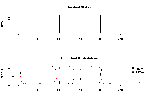
	# http://lipas.uwasa.fi/~bepa/Markov.pdf
	# Expected duration of each regime (1/(1-pii))
	#1/(1-diag(ResFit$HMM$transMat))


	#*****************************************************************
	# It also can be done using depmixS4 package
	#[Getting Started with Hidden Markov Models in R](http://blog.revolutionanalytics.com/2014/03/r-and-hidden-markov-models.html)
	#******************************************************************
	load.packages('depmixS4')

	# Construct and fit a regime switching model
	mod = depmix(y ~ 1, family = gaussian(), nstates = 2, data=data.frame(y=y))
	fm2 = fit(mod, verbose = FALSE)
converged at iteration 69 with logLik: 125.6168
	probs = posterior(fm2)

	layout(1:2)
	plot(probs$state, type='s', main='Implied States', xlab='', ylab='State')

	matplot(probs[,-1], type='l', main='Probabilities', ylab='Probability')
		legend(x='topright', c('State1','State2'),  fill=1:2, bty='n')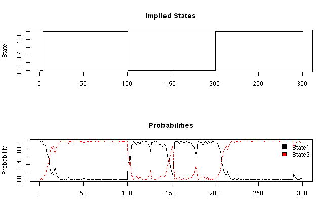
	#*****************************************************************
	# Add some data and see if the model is able to identify the regimes
	#******************************************************************
	bear2  = rnorm( 100, -0.01, 0.20 )
	bull3 = rnorm( 100, 0.10, 0.10 )
	bear3  = rnorm( 100, -0.01, 0.25 )
	true.states = c(true.states, rep(2,100),rep(1,100),rep(2,100))
	y = c( bull1, bear,  bull2, bear2, bull3, bear3 )
	VitPath = RHmm:::viterbi(ResFit, y)$states
DimObs=1
	# map states: sometimes HMMFit function does not assign states consistently
	# let's use following formula to rank states
	# i.e. high risk, low returns => state 2 and low risk, high returns => state 1
	map = rank(sqrt(ResFit$HMM$distribution$var) - ResFit$HMM$distribution$mean)
	VitPath = map[VitPath]

	#*****************************************************************
	# Plot regimes
	#******************************************************************
	data = xts(y, as.Date(1:len(y)))

	layout(1:3)
		plota.control$col.x.highlight = col.add.alpha(true.states+1, 150)
	plota(data, type='h', plotX=F, x.highlight=T)
		plota.legend('Returns + True Regimes')
	plota(cumprod(1+data/100), type='l', plotX=F, x.highlight=T)
		plota.legend('Equity + True Regimes')

		plota.control$col.x.highlight = col.add.alpha(VitPath+1, 150)
	plota(data, type='h', x.highlight=T)
		plota.legend('Returns + Detected Regimes')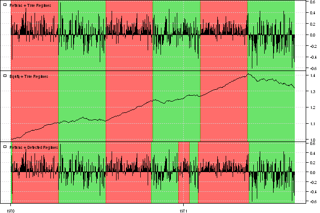
Identifying Changing Market Conditions by Tad Slaff made a great tutorial on Hidden Markov Models using depmixS4 package.
#*****************************************************************
# Load historical prices
#******************************************************************
data = env()
getSymbols('SPY', src = 'yahoo', from = '1970-01-01', env = data, auto.assign = T)

price = Cl(data$SPY)
	open = Op(data$SPY)
ret = diff(log(price))
	ret = log(price) - log(open)

atr = ATR(HLC(data$SPY))[,'atr']


#*****************************************************************
# Construct and fit a regime switching model
#******************************************************************
load.packages('depmixS4')

index = 14:nrow(price)
temp = data.frame(ret=as.vector(ret), atr=as.vector(atr))
	temp = temp[index,]

# We're setting the LogReturns and ATR as our response variables,
# want to set 4 different regimes, and setting the response distributions to be gaussian.
mod = depmix(list(ret~1, atr~1),data=temp,nstates=4,family=list(gaussian(),gaussian()))
fm2 = fit(mod, verbose = FALSE)
converged at iteration 30 with logLik: 18358.98
print(summary(fm2))Initial state probabilties model pr1 pr2 pr3 pr4 0 0 1 0
Transition matrix toS1 toS2 toS3 toS4 fromS1 9.821940e-01 1.629595e-02 1.510069e-03 8.514403e-45 fromS2 1.167011e-02 9.790209e-01 8.775478e-68 9.308946e-03 fromS3 3.266616e-03 8.586650e-47 9.967334e-01 1.350529e-69 fromS4 3.608394e-65 1.047516e-02 1.922545e-130 9.895248e-01
Response parameters Resp 1 : gaussian Resp 2 : gaussian Re1.(Intercept) Re1.sd Re2.(Intercept) Re2.sd St1 2.897594e-04 0.006285514 1.1647547 0.1181514 St2 -6.980187e-05 0.008186433 1.6554049 0.1871963 St3 2.134584e-04 0.005694483 0.4537498 0.1564576 St4 -4.459161e-04 0.015419207 2.7558362 0.7297283
| Re1.(Intercept) | Re1.sd | Re2.(Intercept) | Re2.sd | |
|---|---|---|---|---|
| St1 | 0.000289759401378951 | 0.00628551404616354 | 1.16475474419891 | 0.118151350440916 |
| St2 | -6.98018749098021e-05 | 0.00818643307634358 | 1.65540488736983 | 0.187196307284941 |
| St3 | 0.000213458358141314 | 0.00569448330115608 | 0.453749781945066 | 0.156457606460757 |
| St4 | -0.00044591612667264 | 0.0154192070819596 | 2.75583620018895 | 0.72972830143278 |
probs = posterior(fm2)

print(head(probs))| rownames(x) | state | S1 | S2 | S3 | S4 |
|---|---|---|---|---|---|
| 1 | 3 | 0 | 0 | 1 | 0 |
| 2 | 3 | 0 | 0 | 1 | 0 |
| 3 | 3 | 0 | 0 | 1 | 0 |
| 4 | 3 | 0 | 0 | 1 | 0 |
| 5 | 3 | 0 | 0 | 1 | 0 |
| 6 | 3 | 0 | 0 | 1 | 0 |
layout(1:3)
plota(ret, type='h', col='blue')
	plota.legend('S&P 500 Daily Log Returns', 'blue')
plota(atr, type='l', col='darkgreen')
	plota.legend('Daily ATR(14)', 'darkgreen')

temp = NA * price
	temp[index] = probs$state
plota(temp, type='l', col='darkred')
	plota.legend('Market Regimes', 'darkred')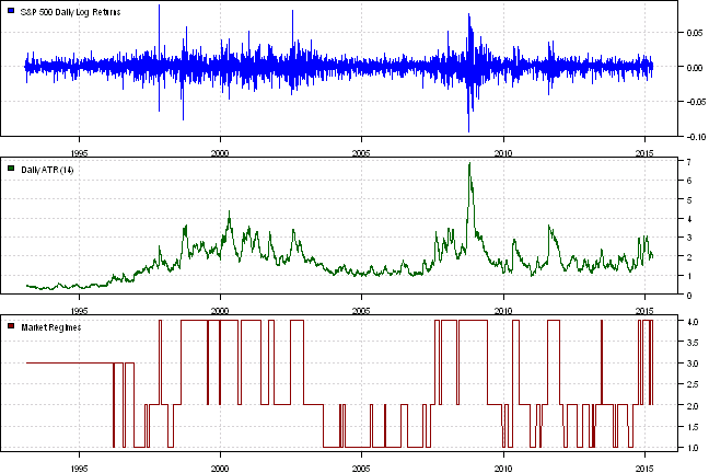
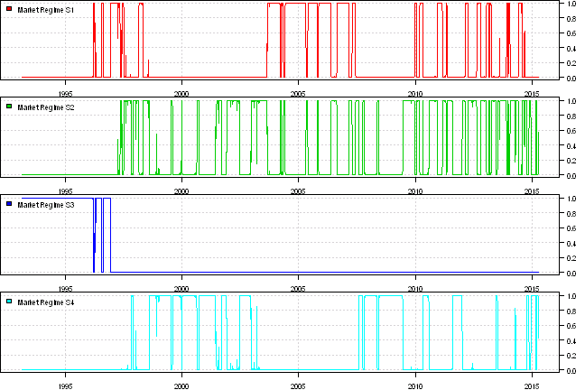
layout(1:4)
for(i in 2:5) {
	temp = NA * price
		temp[index] = probs[,i]
	plota(temp, type='l', col=i)
		plota.legend(paste('Market Regime', colnames(probs)[i]), i)
}
Please note that solution changes each time you run the above code.
(this report was produced on: 2015-04-17)