RFinance 2015
29 May 2015To install Systematic Investor Toolbox (SIT) please visit About page.
Following is code and plots used in RFinance 2015 presentation.
We will use a C++ function to compute Lagged Correlations from the Run Leadership Rcpp post.
First, let’s load historical prices for S&P 500. Please note that we are using current companies in the S&P 500 index and assume the index composition does not change.
Please note we moved lagged correlation logic to RcppParallel in order to finish computations in reasonable time. There are 37B correlation computations 37,724,400,000 = 124,750 * 120 * 2,520
- For Each Pair in SP500 = 500 * 499 / 2 = 124,750
- 120 look back window = (+)60 lag and (-)60 lag = 120 correlation
- 10 year = 10 * 252 = 2,520
To run the code below please make sue you have the lead.lag.correlation.cpp file downloaded lead.lag.correlation.cpp.
#*****************************************************************
# Load historical end of day data
#*****************************************************************
library(SIT)
load.packages('quantmod')

filename = 'big.test.Rdata'
prices = load.test.data(filename)
	tickers = colnames(prices)

# please note that using raw price time series introduces too much noise
# in the lagged correlation computations, transforming data with 5 period EMA
# make lagged correlation computations more stable
sma = bt.apply.matrix(prices, EMA, 5)

#*****************************************************************
# Compile Run-Lead-Lag function
#*****************************************************************
# make sure to install [Rtools on windows](http://cran.r-project.org/bin/windows/Rtools/)
load.packages('Rcpp')
load.packages('RcppParallel')

# load Rcpp functions
sourceCpp('lead.lag.correlation.cpp')

#*****************************************************************
# Two Time Series and Lagged Correlation
#*****************************************************************
nwindow = 120
hist.data = prep.test.data(sma, '2014-05-16', nwindow)

# compute leadership, call Rcpp function
lead.lag.cor = cp_run_leadership_smart(hist.data, nwindow, T)

threshold = 0.75
leaders = get.leaders(lead.lag.cor, nwindow, threshold, tickers)

# find high correlation pair i = "VRSN", j = "OMC"
i = names(leaders)[1]
	adj.mat = lead.lag.cor[,,nwindow]
		rownames(adj.mat) = colnames(adj.mat) = tickers
j = names(which.max(adj.mat[i,]))

# look at details
out = rtest.one(hist.data, nwindow, i, j)

# plot lagged correlation
rtest.visualize(out)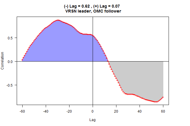
# plot time series side by side
rtest.visualize.relationship(out)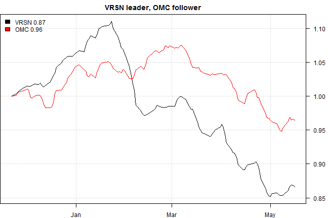
#*****************************************************************
# Leadership discovery graph
#*****************************************************************
index = match(spl('C,BAC,JPM,BK'), tickers)

nwindow = 120
hist.data = prep.test.data(sma[,index], '2014-05-16', nwindow)

# compute leadership, call Rcpp function
lead.lag.cor = cp_run_leadership_smart(hist.data, nwindow, T)

threshold = 0.2
leaders = get.leaders(lead.lag.cor, nwindow, threshold, tickers[index], T)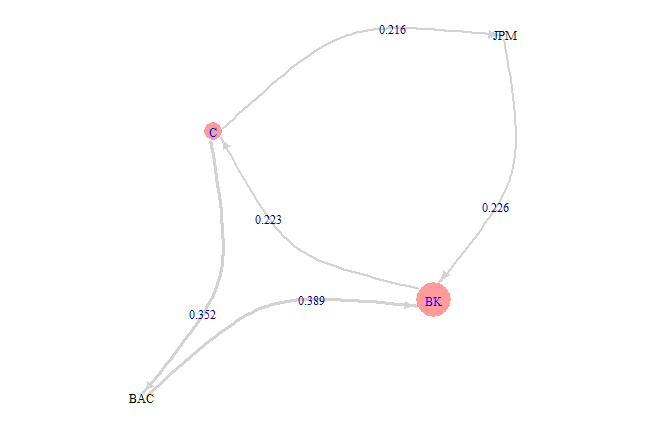
The Algorithm has following parameters:
- nwindow - length of the look back window
- nlag - lag used in the lagged correlation computations, assumed to be half of look back window
- threshold - correlation threshold used to remove edges from the graph
#*****************************************************************
# Sensitivity of Parameters:
#*****************************************************************

# compute leaders for various parameters
windows = c(30,60,90,120,180)
thresholds = seq(0.2, 0.8, by=0.05)
hist.data = prep.test.data(sma, '2014-05-16', max(windows))
	nperiod = nrow(hist.data)

out = list()
for(nwindow in windows) {
	lead.lag.cor = cp_run_leadership_smart(last(hist.data, nwindow), nwindow, T)
	for(threshold in thresholds)
		out[[paste(nwindow, threshold)]] = get.leaders(lead.lag.cor, nwindow, threshold, tickers)
}


# plot: #leaders vs correlation threshold for various window lengths
temp = matrix(NA, nr=len(thresholds), nc=len(windows))
for(i in 1:len(windows))
	for(j in 1:len(thresholds))
		temp[j,i] = len(out[[paste(windows[i], thresholds[j])]])


matplot.helper(temp, thresholds, 'Correlation Threshold', 'Number of Leaders', 'topleft', windows, 'Number of Leaders')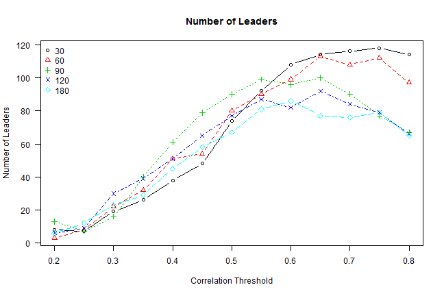
# plot: containment rate of leaders vs correlation threshold for various window lengths
# containment rate of leaders = [Leader(g) intersect Leader(g-1)] / Leader(g-1)
temp = matrix(1, nr=len(thresholds), nc=len(windows))
for(i in 1:len(windows))
	for(j in 2:len(thresholds)) {
		g0 = names(out[[paste(windows[i], thresholds[j-1])]])
		g1 = names(out[[paste(windows[i], thresholds[j])]])
		temp[j,i] = len(intersect(g0, g1)) / len(g0)
	}

matplot.helper(temp, thresholds, 'Correlation Threshold', 'Containment Rate of Leaders', 'topright', windows, 'Containment Rate of Leaders')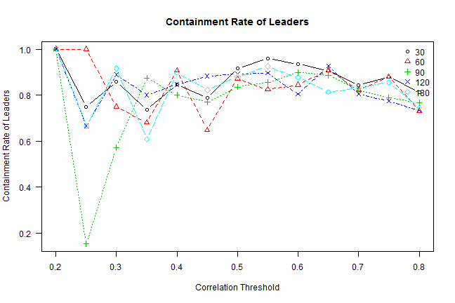
Next let’s see how stable the leaders selected from one period to the next one.
#*****************************************************************
# Compute leaders; need to split it history into years; otherwise run out of memory
#*****************************************************************
leader.filename = 'leaders.Rdata'

nwindow = 120
threshold = 0.6

if(!file.exists(leader.filename)) {
	out = list()
	index = index(prices)
	for(y in 2001:2015) {
		hist.data = prep.test.data(sma, paste(y), nwindow)
		nperiod = nrow(hist.data)

		offset = match(index(hist.data)[1], index) - 1
		cat(nwindow+offset, nperiod+offset, 'index \n')

		cat(y, 'Leader ship \n')
		lead.lag.cor = cp_run_leadership_smart(hist.data, nwindow, T)

		cat(y, 'Extract leader\n')
		for(i in nwindow:nperiod)
			out[[i + offset]] = get.leaders(lead.lag.cor, i, threshold, tickers)

		gc(T)
	}

	save(out, file='leaders.Rdata')
}

#*****************************************************************
# Stability of Leaders Over Time:
# [Leader(t1) intersect Leader(t0)] / [Leader(t1) union Leader(t0)]
#*****************************************************************
load(leader.filename)
nperiod = nrow(prices)
nstart = max(which(sapply(out, len) == 0))+1

temp = array(NA, nperiod)
for(i in (nstart+1):nperiod) {
	g0 = names(out[[i-1]])
	if(!is.null(g0)) {
		g1 = names(out[[i]])
		temp[i] = len(intersect(g0, g1)) / len(union(g0, g1))
	}
}

# Containment Rate = [Leader(t1) intersect Leader(t0)] / [Leader(t1) union Leader(t0)]
temp = make.xts(temp, index(prices))
plota(temp, type='l', ylim=c(0.5,1), col='gray')
	plota.lines(EMA(temp, 50), col='black', lwd=2)
	plota.legend('Containment Rate of Leaders,50 SMA','gray,black')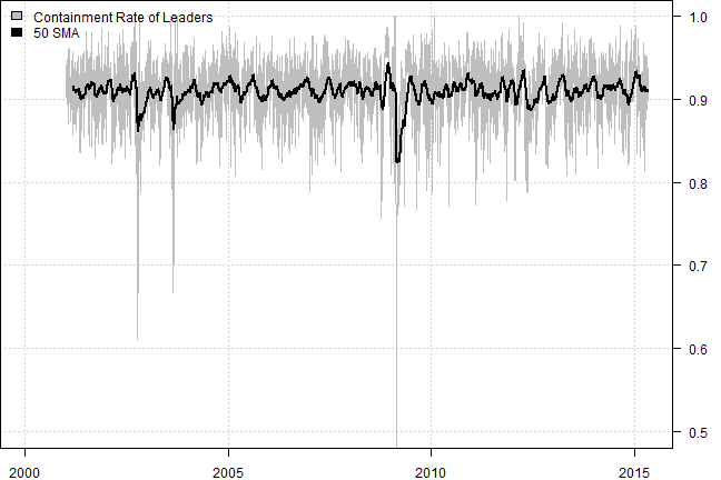
# Number of Leaders
temp = sapply(out, len)
	temp[temp == 0] = NA
temp = make.xts(temp, index(prices))

plota(temp, type='l', col='gray')
	plota.lines(EMA(temp, 50), col='black', lwd=2)
	plota.legend('Number of Leaders,50 SMA','gray,black')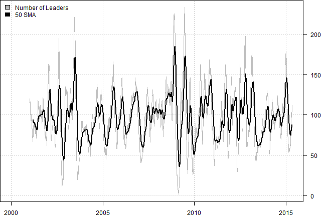
Create Leadership index. Leadership index is the subset of companies in the S&P 500 that are leaders as determined by the Algorithm above. We will create two versions of leadership index:
- equal weight leadership index
- leadership index weighted proportional to the PageRank score
#*****************************************************************
# Create Leadership index
#*****************************************************************
data = env(
	symbolnames = tickers,
	dates = index(prices),
	fields = 'Cl',
	Cl = prices)
bt.prep.matrix(data)


models = list()
data$weight[] = NA
  data$weight[nstart:nperiod,] = 1/len(tickers)
models$SP500 = bt.run.share(data, clean.signal=F, silent=T)

# Leadership index
data$weight[] = 0
	for(i in nstart:nperiod)
		data$weight[i, names(out[[i]])] = 1 / len(out[[i]])
models$leader.ew = bt.run.share(data, clean.signal=F, silent=T)

data$weight[] = 0
	for(i in nstart:nperiod)
		data$weight[i, names(out[[i]])] = out[[i]] / sum(out[[i]])
models$leader.pagerank = bt.run.share(data, clean.signal=F, silent=T)

plotbt(models, plotX = T, log = 'y', LeftMargin = 3, main = NULL)
	mtext('Cumulative Performance', side = 2, line = 1)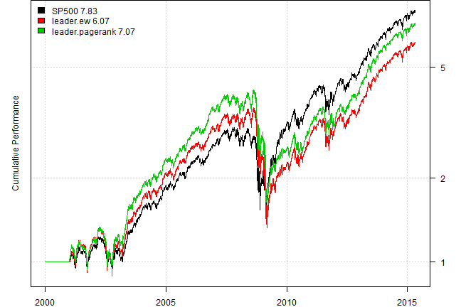
Next use Leadership index to time allocation to S&P 500, if leadrship index is above 100 period average allocate to the S&P 500; otherwise stay in cash.
#*****************************************************************
# Timing Back-tests based on leadership index
#*****************************************************************
data.eq = env()
for(m in names(models))
	data.eq[[m]] = make.stock.xts(models[[m]]$equity)
bt.prep(data.eq)

frequency = 'months'
period.ends = endpoints(data.eq$prices, frequency)
  period.ends = period.ends[period.ends > 0]

sma = bt.apply.matrix(data.eq$prices, SMA, 100)

models.eq = list()

data.eq$weight[] = NA
	data.eq$weight[period.ends, 'SP500'] = iif((data.eq$prices > sma)[period.ends, 'SP500'], 1, 0)
models.eq$ew.timing = bt.run.share(data.eq, clean.signal=T, silent=T)

data.eq$weight[] = NA
	data.eq$weight[period.ends, 'SP500'] = iif((data.eq$prices > sma)[period.ends, 'leader.ew'], 1, 0)
models.eq$ew.leader.timing = bt.run.share(data.eq, clean.signal=T, silent=T)

data.eq$weight[] = NA
	data.eq$weight[period.ends, 'SP500'] = iif((data.eq$prices > sma)[period.ends, 'leader.pagerank'], 1, 0)
models.eq$ew.leader.pagerank.timing = bt.run.share(data.eq, clean.signal=T, silent=T)

plotbt(models.eq, plotX = T, log = 'y', LeftMargin = 3, main = NULL)
	mtext('Cumulative Performance', side = 2, line = 1)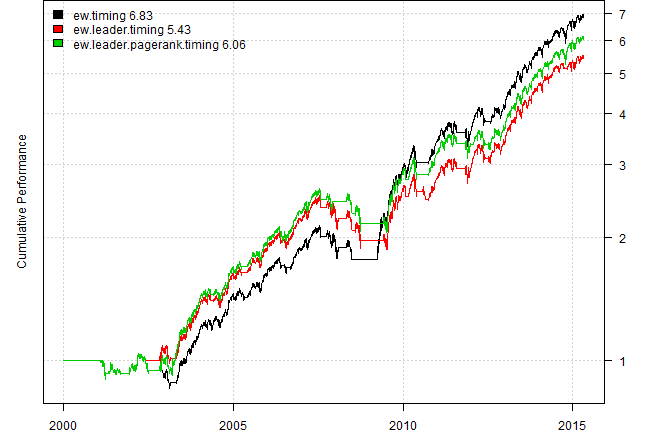
plotbt.strategy.sidebyside(models.eq, make.plot=T, return.table=F, perfromance.fn=engineering.returns.kpi)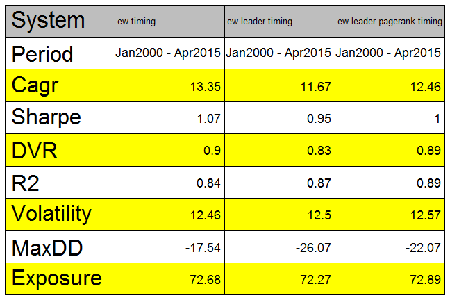
#plotbt.custom.report.part1(models.eq)
#strategy.performance.snapshoot(bt.trim(models.eq), T)
Unfortunately, we do not observe any predictive power of using leadership index versus just using S&P 500 index.
In the future work we want to concentrate on:
- better matching time series with dynamic time wrapping (DTW) - it will be more computationally intensive
- consider negative correlation in graph construction
- testing on intraday data. probably there is a better chance to capture intraday leadership because price action during 120 minutes might be more relevant than price action over 120 days. I.e. market react and adjusts with in minutes, not days or weeks
Thank you and looking forward to meeting you at RFinance.
Supporting functions:
#*****************************************************************
# Load historical end of day data
#*****************************************************************
load.test.data = function(filename) {
	if(!file.exists(filename)) {
	  #tickers = nasdaq.100.components()
	  tickers = sp500.components()$tickers

	  data = env()
	  getSymbols.extra(tickers, src = 'yahoo', from = '1970-01-01', env = data, auto.assign = T)

		rm.index = which(sapply(ls(data), function(i) is.null(data[[i]])))
		if(any(rm.index)) env.del(names(rm.index), data)

	  for(i in ls(data)) data[[i]] = adjustOHLC(data[[i]], use.Adjusted=T)
	  #print(bt.start.dates(data))

	  bt.prep(data, align='keep.all', dates='2000::', fill.gaps=T)

	  # remove ones with little history
	  prices = data$prices
	  bt.prep.remove.symbols(data, which(
   		count(prices, side = 2) < 3*252 | is.na(last(prices))
	  ))

	  # show the ones removed
	  print(setdiff(tickers,names(data$prices)))

	  prices = data$prices
	  save(prices, file=filename)
	}
	load(file=filename)
	prices
}


#*****************************************************************
# Extract Subset of data
#*****************************************************************
prep.test.data = function(prices, index, nwindow, use.price = T) {
	index = dates2index(prices, index)
	hist.data = iif(use.price, prices, prices / mlag(prices) - 1)

	index = range(index)
	index[1] = iif(index[1] < nwindow, 1, index[1] - nwindow + 1)
	hist.data[index[1]:index[2],,drop=F]
}


#*****************************************************************
# Extract Leaders
#*****************************************************************
get.leaders = function(lead.lag.cor, index, threshold, tickers, make.plot=F) {
	# create adjacency matrix
	adj.mat = lead.lag.cor[,,index]
		rownames(adj.mat) = colnames(adj.mat) = tickers
		adj.mat = clean.adj(adj.mat, threshold)
	if(nrow(adj.mat) == 0) return(c());

	# construct graph
	load.packages('igraph')
	g  = graph.adjacency(adj.mat,weighted=TRUE)
		#basic.graph.plot(g)
		#sort(page.rank(g, directed = TRUE)$vector, decreasing = T)

	# extract leaders
	leaders = extract.leaders(g, adj.mat)
	if(make.plot) advanced.graph.plot(g, leaders)
	leaders
}

# remove zero entries
clean.adj = function(adj.mat, threshold = 0.5) {
	adj.mat[ abs(adj.mat) < threshold] = 0
	adj.mat[ is.na(adj.mat)] = 0
	keep.index = (rowSums(adj.mat != 0) >= 1) | (colSums(adj.mat != 0) >= 1)
	adj.mat = adj.mat[keep.index, keep.index]
	adj.mat
}

# remove descendants
remove.descendant = function(j, stack) {
	if(j == stack$n) return()

	for(i in (j+1):stack$n)
		if(stack$index[i])
			if(stack$adj.mat[stack$L[i],stack$L[j]] != 0) {
				remove.descendant(i, stack)
				stack$index[i] = F
			}
}

extract.leaders = function(g, adj.mat) {
	# compute page rank vector
	p = page.rank(g, directed = TRUE)$vector

	# sort time series in descending order by page.rank
	L = sort.list(p, decreasing = T)
	#L = names(sort(p, decreasing = T))

	# temp var to be used in remove.descendant function
	n = len(p)
	stack = env(index = rep(T, n), n, adj.mat, L)

	for(i in 1:n)
		if(stack$index[i])
			remove.descendant(i, stack)
	leaders = p[L[stack$index]]
	leaders
}

#*****************************************************************
# Visualize Graph
#*****************************************************************
basic.graph.plot = function(g) {
	par(mar=c(0,0,0,0))
	#V(g)$label.cex = 0.5
	plot(g, edge.label=round(E(g)$weight, 3), edge.label.cex = 0.5, edge.width = 1,
		edge.arrow.size = 0.5,edge.color = 'lightgray', edge.curved=T,
		vertex.label.cex = 0.5,	vertex.size=5, vertex.color=NA, vertex.frame.color=NA)
}

advanced.graph.plot = function(g, leaders) {
	# plot leaders
	col = iif(is.na(match(V(g)$name, names(leaders))), 'white', 'red')
	label.col = iif(is.na(match(V(g)$name, names(leaders))), 'black', 'blue')
	size = leaders[match(V(g)$name, names(leaders))]
		size = punif(size, min=min(leaders), max=max(leaders))
		size = iif(is.na(size), 5, round(10*(size+1)))

	par(mar=c(0,0,0,0))
	plot(g, edge.label=round(E(g)$weight, 3), edge.label.cex = 1, edge.width = 10*E(g)$weight,
		edge.arrow.size = 0.85,edge.color = 'lightgray', edge.curved=T,
		layout=layout.fruchterman.reingold,
		vertex.color=col.add.alpha(col,100),
		vertex.label.color = label.col,
		vertex.label.cex = 1,	vertex.size=size, vertex.color=NA, vertex.frame.color=NA)
}

#*****************************************************************
# Lagged correlation for given two entries
#*****************************************************************
rtest.one = function(ret, nwindow, c1.name, c2.name) {
	c1 = which(colnames(ret) == c1.name)
	c2 = which(colnames(ret) == c2.name)
	if(c1 < c2) { # switch
		temp = c2; c2 = c1; c1 = temp
		temp = c2.name; c2.name = c1.name; c1.name = temp
	}

	nlag = floor(nwindow/2)
	n = ncol(ret)
	nperiod = nrow(ret)
	out = array(NA, c(n,n,nperiod))
	index = !lower.tri(out[,,1])

	i = nperiod

		temp = coredata(ret[(i-nwindow+1):i,])
		temp.out = matrix(NA, n,n)

			data1 = temp[,c1]
			data2 = temp[,c2,drop=F]

			# c2 leader, c1 follower, because c1 always ends at nwindow
			c1.cor = c()
			for (lag in 0:nlag) {
				cor.temp = cor(data1[(lag+1):nwindow], data2[1:(nwindow-lag),])
				c1.cor = c(c1.cor, cor.temp)
			}

			# c1 leader, c2 follower, because c2 always ends at nwindow
			c2.cor = c()
			for (lag in 1:nlag) {
				cor.temp = cor(data1[1:(nwindow-lag)], data2[(lag+1):nwindow,])
				c2.cor = c(c2.cor, cor.temp)
			}


			c1.cor.mean = sum(pmax(c1.cor,0)) / (nlag + 1)
			c2.cor.mean = sum(pmax(c2.cor,0)) / nlag
			# if c1.cor >= c2.cor hence c2 leader, c1 follower i.e. cor(data1[(lag+1):nwindow], data2[1:(nwindow-lag),])
			# if c2.cor >= c1.cor hence c1 leader, c2 follower i.e. cor(data1[1:(nwindow-lag)], data2[(lag+1):nwindow,])
			relationship = iif(c1.cor.mean >= c2.cor.mean, 'c2 leader, c1 follower', 'c1 leader, c2 follower')
			relationship = gsub('c1', c1.name, gsub('c2', c2.name, relationship))
		list(
			c1 = c1, c2 = c2, c1.name = c1.name, c2.name = c2.name,
			x = -nlag:nlag,
			y = c(rev(c2.cor), c1.cor),
			c1.cor = to.nice(c1.cor.mean),
			c2.cor = to.nice(c2.cor.mean),
			relationship = relationship,
			c1.ret = ret[(i-nwindow+1):i,c1],
			c2.ret = ret[(i-nwindow+1):i,c2]

		)
}

#*****************************************************************
# Visualize results
#*****************************************************************
rtest.visualize = function(out) {
	par(mar=c(5,4,4,5))
	plot(out$x, out$y, type = "n", xlab='Lag', ylab='Correlation', las=1,
		main = paste('(-) Lag =', out$c2.cor, ', (+) Lag =', out$c1.cor,
		'\n', out$relationship)
	)

	col1 = col.add.alpha('blue',100)
	polygon(c(first(out$x), out$x, last(out$x)), c(0, pmax(out$y,0), 0), col=col1, border=col1)

	col1 = col.add.alpha('gray',200)
	polygon(c(first(out$x), out$x, last(out$x)), c(0, pmin(out$y,0), 0), col=col1, border=col1)

	abline(h=0, v=0)
	lines(out$x, out$y, col='red')
	lines(out$x, out$y, type='b', pch='+', col='red')
}

rtest.visualize.relationship = function(out, is.ret=F) {
	if(is.ret) {
		temp = cbind(cumprod(1 + out$c1.ret), cumprod(1 + out$c2.ret))
		colnames(temp) = c(out$c1.name, out$c2.name)
	} else
		temp = cbind(out$c1.ret, out$c2.ret)

	plota.matplot(scale.one(temp), main=out$relationship)
}

matplot.helper = function(mat, x=1:nrow(mat), xlab='', ylab='', legend='topleft', y=1:ncol(mat), main='') {
	col = 1:ncol(mat)
	matplot(x, mat, type='b', pch=col, xlab=xlab, ylab=ylab, las=1, main=main)
	legend(legend, legend=y, col=col, pch=col, bty='n')
}
(this report was produced on: 2015-05-25)