Optimize Trading System
04 Feb 2015To install Systematic Investor Toolbox (SIT) please visit About page.
There is a great example of htmlwidgets in the Interactive Parallel Coordinates. You can interactively manipulate the Parallel Coordinates Plot to zoom in on interesting observations.
Sometime ago, I was reading about Visualizing system parameter optimization results at Visualizing Data. The article was using XDat app to create and manipulate back-test results.The idea is to run multiple back tests by varying system parameters, and display results using Parallel Coordinates plot.
A great example of system parameter optimization is described at How to optimize trading system. The article presents a 3 dimensional plot with one parameter on X axis, one parameter on Y axis, and CAGR on the Z axis. This is a very good approach if you only optimize two parameters, but what to do if you have more than two parameters?
The Parallel Coordinates come to the rescue. Let’s say we run a
system parameter optimization, varying 3 parameters and stored
results in the data matrix. The first column will contain CAGR
and columns 2:4 will contain parameters values.
For example:
#*****************************************************************
# Load historical data
#*****************************************************************
library(SIT)
load.packages('quantmod')

tickers = 'SPY'

data <- new.env()
getSymbols(tickers, src = 'yahoo', from = '1970-01-01', env = data, auto.assign = T)
for(i in ls(data)) data[[i]] = adjustOHLC(data[[i]], use.Adjusted=T)
bt.prep(data, align='remove.na')


#*****************************************************************
# Setup
#*****************************************************************
prices = data$prices

# all possible combinations
choices = expand.grid(
	fast=seq(5, 50, by = 5),
 mid=seq(10, 80, by = 10),
 slow=seq(60, 200, by = 20),
KEEP.OUT.ATTRS=F)

# only select fast < mid < slow
choices = choices[choices$fast < choices$mid & choices$mid < choices$slow,]

# pre compute all moving averages
mas = list()
for( i in unique(unlist(choices)) )
	mas[[i]] = bt.apply.matrix(prices, SMA, i)

# run back test over all combinations
result = choices
	result$CAGR = NA
nyears = compute.nyears(data$prices)

for(i in 1:nrow(choices)) {
	signal = iif(mas[[choices$fast[i]]] > mas[[choices$mid[i]]] &
 	mas[[choices$mid[i]]] > mas[[choices$slow[i]]], 1,
 	iif(mas[[choices$fast[i]]] > mas[[choices$slow[i]]] &
  	mas[[choices$mid[i]]] > mas[[choices$slow[i]]], 0.5, 0))

	data$weight[] = NA
		data$weight[] = signal
	model = bt.run.weight.fast(data)
	result$CAGR[i] = compute.cagr(model$equity, nyears)
	#model = bt.run(data, silent=T)
	#result$CAGR[i] = model$cagr
}

# re-arrange
result = result[,spl('CAGR,slow,mid,fast')]

#*****************************************************************
# Parallel Coordinates Plot
# http://www.statmethods.net/advgraphs/interactive.html
# http://stackoverflow.com/questions/3942508/implementation-of-parallel-coordinates
# http://www.r-statistics.com/tag/parallel-coordinates/
#*****************************************************************
library(MASS)
parcoord(result, var.label=T, col=1:nrow(result))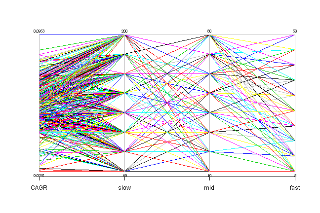
It is quite hard to navigate this plot.
Ideally, you would want to select a ranges for parameters and check corresponding system CAGRs, or alternatively select a range of CAGRs and see what parameters produced them. The amazing Acinonyx - iPlots eXtreme package allows this Interactivity.
#*****************************************************************
# Interactive Parallel Coordinates Plot
# Please
#*****************************************************************
library(Acinonyx)
ipcp(result)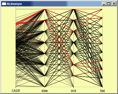
Another way is to achieve this interactive behaviour is to use a great example of htmlwidgets in the Interactive Parallel Coordinates.
(this report was produced on: 2015-02-06)