Moving Average

22 Feb 2015

To install Systematic Investor Toolbox (SIT) please visit About page.

The Quantitative Approach To Tactical Asset Allocation Strategy(QATAA) by Mebane T. Faber model is using 10 month moving average as a filter to switch strategy to cash. If at the month end the asset’s price is above the moving average, it gets allocation; otherwise it’s allocation goes to cash.

The initial question i wanted to answer is what so special about 10 months; and why does 10 is constant for all assets and regimes. I played with idea of adjusting moving average look back based on the historical volatility. I.e. in periods of high volatility, the shorter moving average will take us from the market faster, while in low volatility, the longer moving average will keep us in the markets regardless of the whipsaws. Unfortunately, it resulted in higher turnover and worse results.

The good part is that i spend some time analyzing the base 10 month moving average strategy and seeing quite whipsaw, the simple fix is to use +/- 5% bands around 10 month moving average to reduce whipsaw, reduce turnover and increase returns.

Below I will show how this concept works:

#*****************************************************************
# Load historical data
#*****************************************************************
library(SIT)
load.packages('quantmod')

# load saved Proxies Raw Data, data.proxy.raw, to extend DBC and SHY
# please see http://systematicinvestor.github.io/Data-Proxy/ for more details
load('data/data.proxy.raw.Rdata')

tickers = '
SPY
CASH = SHY + TB3Y
'

data <- new.env()
getSymbols.extra(tickers, src = 'yahoo', from = '1970-01-01', env = data, raw.data = data.proxy.raw, set.symbolnames = T, auto.assign = T)
for(i in data$symbolnames) data[[i]] = adjustOHLC(data[[i]], use.Adjusted=T)
bt.prep(data, align='remove.na', fill.gaps = T)

#*****************************************************************
# helper function to visualize signal
#*****************************************************************
cash.visualize.signal = function(model = spl('base,bands'), dates='::') {
  model = model[1]
  
  signal = iif(model == 'base', prices > sma,
    iif(cross.up(prices, sma * 1.05), 1, iif(cross.dn(prices, sma * 0.95), 0, NA))
  )$SPY
  
  signal[] = ifna( ifna.prev(signal), 0)

  # create a model based on signal
  data$weight[] = NA
    data$weight$SPY = signal
    data$weight$CASH = 1 - ifna( ifna.prev(data$weight$SPY), 0)
  model = bt.run.share(data, clean.signal=T, silent=T)

  # create a plot to visualize signal
  p = prices$SPY
  p1 = sma$SPY
  e = model$equity
  w = model$weight$SPY
  highlight = (signal==1)[dates]

  layout(1:4)
  plota(p[dates] ,type='l', plotX=F, x.highlight = highlight)
    plota.lines(p1 ,type='l', col='blue')
    if(model == 'base')
      plota.legend('SPY,sma','black,blue')
    else {
      plota.lines(1.05*p1 ,type='l', col='green')
      plota.lines(0.95*p1 ,type='l', col='green')
      plota.legend('SPY,sma,sma bands','black,blue,green')
    }
  
  plota( 100 * EMA(compute.drawdown(p),20)[dates] ,type='l', plotX=F, x.highlight = highlight)  
    plota.lines( 100 * EMA(compute.drawdown(e),20)[dates] ,col='blue')
    plota.legend('SPY drawdown,Model drawdown', 'black, blue')                                                                                                   
  
  plota( 100 * EMA(p/mlag(p,252)[dates]-1,20) ,type='l', x.highlight = highlight, plotX=F)
    abline(h=0, col='red')
    plota.lines( 100 * EMA(e/mlag(e,252)[dates]-1,20) ,col='blue')            
    plota.legend('SPY 12M return, Model  12M return','black,blue')                       

  plota(w[dates] ,type='s', x.highlight = highlight)
    plota.legend('weight')
    
  #iline(remove.col='green')
}

prices = data$prices
sma = bt.apply.matrix(prices, SMA, 10*22)
cash.visualize.signal('base', '2000::2001')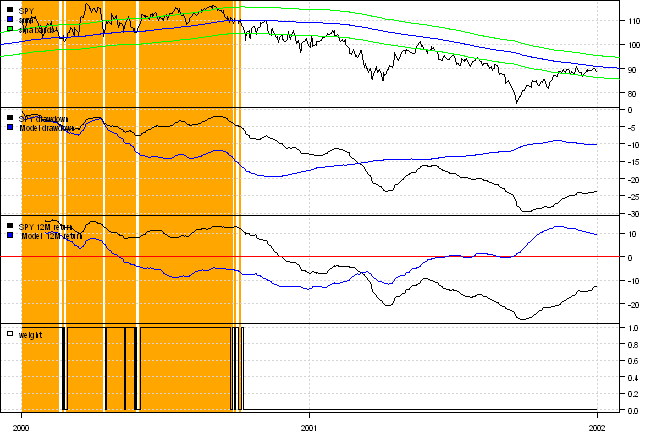

plot of chunk plot-2

cash.visualize.signal('bands', '2000::2001')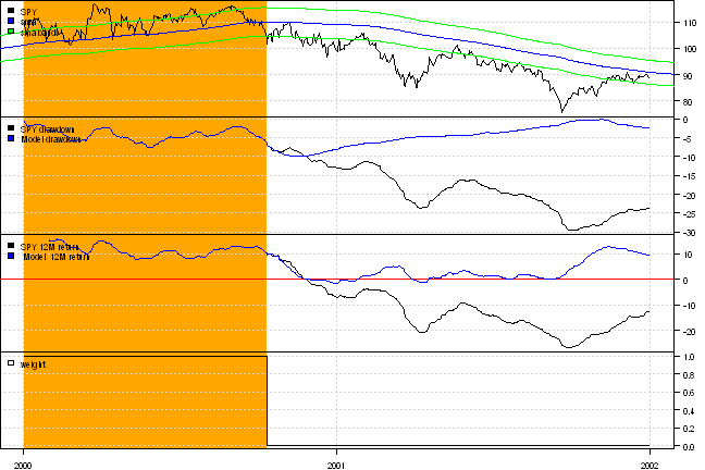

plot of chunk plot-2

The benefit of delay entry / exit is less trades, smaller turnover and hopefully better returns if whipsaws outweigh decrease in performance due to delay’s

#*****************************************************************
# Setup
#*****************************************************************
prices = data$prices

models = list()

#*****************************************************************
# SPY
#******************************************************************
data$weight[] = NA
  data$weight$SPY = 1
models$SPY = bt.run.share(data, clean.signal=T, trade.summary=T, silent=T)

#*****************************************************************
# SPY + 10 month go to cash filter
#******************************************************************
sma = bt.apply.matrix(prices, SMA, 10*22)
 
data$weight[] = NA
  data$weight$SPY = iif(prices$SPY > sma$SPY, 1, 0)
  data$weight$CASH = 1 - ifna( ifna.prev(data$weight$SPY), 0)
models$SPY.CASH = bt.run.share(data, clean.signal=T, trade.summary=T, silent=T)

#*****************************************************************
# SPY + 10 month +5/-5% go to cash filter
#******************************************************************
data$weight[] = NA
  data$weight$SPY = iif(cross.up(prices, sma * 1.05), 1, iif(cross.dn(prices, sma * 0.95), 0, NA))$SPY
  data$weight$CASH = 1 - ifna( ifna.prev(data$weight$SPY), 0)
models$SPY.CASH.BAND = bt.run.share(data, clean.signal=T, trade.summary=T, silent=T)

I also included my attempts at dynamic look back moving average, but in this form it is not useful.

#*****************************************************************
# SPY + dynamic cash filter base on volatility
#******************************************************************
ret = diff(log(prices))
hist.vol = bt.apply.matrix(ret, runSD, n = 21)

vol.rank = bt.apply.matrix(hist.vol, percent.rank, 252)

sma.cash = sma * NA
sma.cash[] = iif(vol.rank < 0.5, bt.apply.matrix(prices, SMA, 10*22), bt.apply.matrix(prices, SMA, 1*22))

data$weight[] = NA
  data$weight$SPY = iif(prices$SPY <= sma$SPY | prices$SPY <= sma.cash$SPY, 0, iif(prices$SPY > sma$SPY, 1, NA))
  data$weight$CASH = 1 - ifna( ifna.prev(data$weight$SPY), 0)
models$SPY.CASH.VOL.SIMPLE = bt.run.share(data, clean.signal=T, trade.summary=T, silent=T)

#*****************************************************************
# SPY + dynamic cash filter base on volatility; multiple levels
#******************************************************************
nbreaks = 5
map.index = seq(0,1, 1/nbreaks)
map = bt.apply.matrix(vol.rank, function(x) as.numeric(cut(x, map.index)))

sma.cash = sma * NA
for(i in 1:nbreaks) {
	temp = coredata(bt.apply.matrix(prices, SMA, (nbreaks - i + 1)* 2 *22))
	index = ifna(map == i, F)
	sma.cash[index] = temp[index]
}

data$weight[] = NA
  data$weight$SPY = iif(prices$SPY <= sma$SPY | prices$SPY <= sma.cash$SPY, 0, iif(prices$SPY > sma$SPY, 1, NA))
  data$weight$CASH = 1 - ifna( ifna.prev(data$weight$SPY), 0)
models$SPY.CASH.VOL = bt.run.share(data, clean.signal=T, trade.summary=T, silent=T)

#*****************************************************************
# Report
#*****************************************************************
#strategy.performance.snapshoot(models, T)
plotbt(models, plotX = T, log = 'y', LeftMargin = 3, main = NULL)
	mtext('Cumulative Performance', side = 2, line = 1)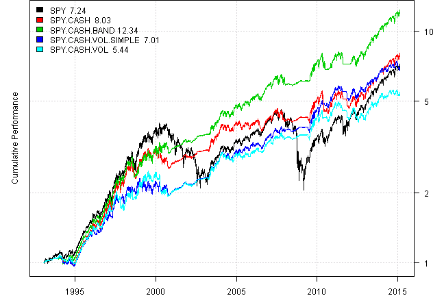

plot of chunk plot-4

print(plotbt.strategy.sidebyside(models, make.plot=F, return.table=T,perfromance.fn = engineering.returns.kpi))

	SPY	SPY.CASH	SPY.CASH.BAND	SPY.CASH.VOL.SIMPLE	SPY.CASH.VOL
Period	Jan1993 - Feb2015	Jan1993 - Feb2015	Jan1993 - Feb2015	Jan1993 - Feb2015	Jan1993 - Feb2015
Cagr	9.4	9.9	12.1	9.2	8
DVR	41.9	78.3	91.4	83.8	74
Sharpe	56.7	83.6	97.1	90.8	77.1
R2	73.9	93.7	94.1	92.3	96
Win.Percent	100	41.1	100	45.7	43.3
Avg.Trade	623.7	1.9	27.6	0.7	0.7
MaxDD	-55.2	-20.1	-19.1	-15.9	-22.3
Num.Trades	1	146	12	302	254

layout(1)
barplot.with.labels(sapply(models, compute.turnover, data), 'Average Annual Portfolio Turnover')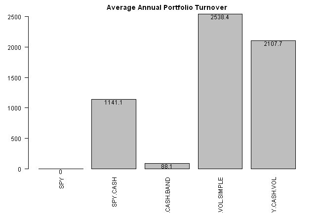

plot of chunk plot-4

Next, let’s apply same bands logic to the TAA model:

tickers = '
US.STOCKS = VTI + VTSMX
FOREIGN.STOCKS = VEU + FDIVX
US.10YR.GOV.BOND = IEF + VFITX
REAL.ESTATE = VNQ + VGSIX
COMMODITIES = DBC + CRB
CASH = BND + VBMFX,
SP500 = SPY
'

# load saved Proxies Raw Data, data.proxy.raw
load('data/data.proxy.raw.Rdata')

data <- new.env()

getSymbols.extra(tickers, src = 'yahoo', from = '1970-01-01', env = data, raw.data = data.proxy.raw, auto.assign = T, set.symbolnames = T)
  for(i in data$symbolnames) data[[i]] = adjustOHLC(data[[i]], use.Adjusted=T)
bt.prep(data, align='remove.na')


#*****************************************************************
# Setup
#*****************************************************************
data$universe = data$prices > 0
	# do not allocate to CASH
	data$universe$CASH = NA 
  data$universe$SP500 = NA

prices = data$prices * data$universe
	n = ncol(prices)

period.ends = endpoints(prices, 'months')
  period.ends = period.ends[period.ends > 0]

models = list()

#*****************************************************************
# Benchmarks
#*****************************************************************
data$weight[] = NA
	data$weight$SP500 = 1
models$SP500 = bt.run.share(data, clean.signal=T, trade.summary=T, silent=T)

data$weight[] = NA
	data$weight[period.ends,] = ntop(prices[period.ends,], n)
models$EW = bt.run.share(data, clean.signal=F, trade.summary=T, silent=T)

#*****************************************************************
#The [Quantitative Approach To Tactical Asset Allocation Strategy(QATAA) by Mebane T. Faber](http://mebfaber.com/timing-model/)
#[SSRN paper](http://papers.ssrn.com/sol3/papers.cfm?abstract_id=962461)
#*****************************************************************
sma = bt.apply.matrix(prices, SMA, 10*22)

weight = NA * data$weight

weight = iif(prices > sma, 20/100, 0)
weight$CASH = 1 - rowSums(weight)

data$weight[] = NA
	data$weight[period.ends,] = weight[period.ends,]
models$Model = bt.run.share(data, clean.signal=F, trade.summary=T, silent=T)

#*****************************************************************
# Alternative: MA bands
#*****************************************************************
sma = bt.apply.matrix(prices, SMA, 10*22)
signal = iif(cross.up(prices, sma * 1.05), 1, iif(cross.dn(prices, sma * 0.95), 0, NA))
signal = ifna(bt.apply.matrix(signal, ifna.prev),0)

weight = iif(signal == 1, 20/100, 0)
weight$CASH = 1 - rowSums(weight)

data$weight[] = NA
	data$weight[period.ends,] = weight[period.ends,]
models$Model.B = bt.run.share(data, clean.signal=F, trade.summary=T, silent=T)

#*****************************************************************
# Report
#*****************************************************************
#strategy.performance.snapshoot(models, T)
plotbt(models, plotX = T, log = 'y', LeftMargin = 3, main = NULL)
	mtext('Cumulative Performance', side = 2, line = 1)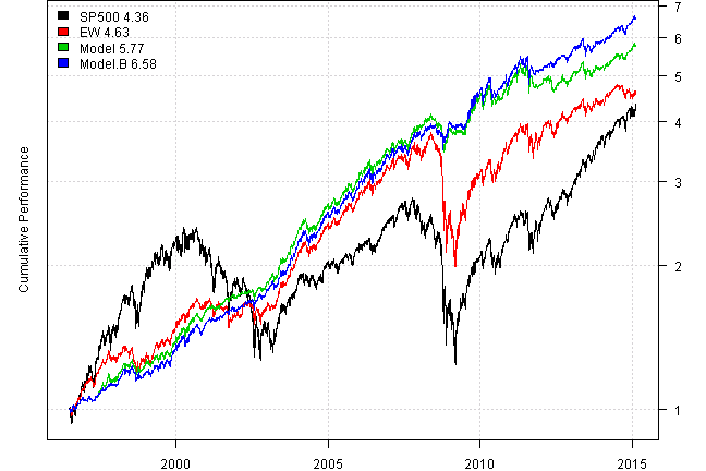

plot of chunk plot-5

print(plotbt.strategy.sidebyside(models, make.plot=F, return.table=T,perfromance.fn = engineering.returns.kpi))

	SP500	EW	Model	Model.B
Period	Jun1996 - Feb2015	Jun1996 - Feb2015	Jun1996 - Feb2015	Jun1996 - Feb2015
Cagr	8.2	8.6	9.8	10.6
DVR	28.7	64	117.4	127.9
Sharpe	49.2	69.3	120.4	132.7
R2	58.4	92.4	97.5	96.5
Win.Percent	100	59.9	64.4	64.6
Avg.Trade	335.7	0.1	0.2	0.2
MaxDD	-55.2	-47.5	-17.1	-13.1
Num.Trades	1	1113	930	887

layout(1)
barplot.with.labels(sapply(models, compute.turnover, data), 'Average Annual Portfolio Turnover')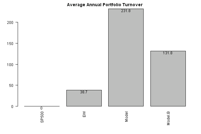

plot of chunk plot-5

The bands logic is easy to implement and it reduced turnover and increase returns.

For other creative ideas on turnover reduction please read Rotational Trading Strategies: borrowing ideas from Engineering Returns post.

(this report was produced on: 2015-02-23)

Systematic Investor's Blog About Contact

Moving Average

Related Posts

RFinance 2016 15 May 2016

Benchmark Plus 14 Apr 2016

Exponentially Weighted Volatility using RCPP 10 Apr 2016