Minimum Spanning Tree
08 Mar 2015To install Systematic Investor Toolbox (SIT) please visit About page.
MKTSTK an another amazing graphics example to visualize correlation matrix at Stock market visualization: Minimum Spanning Trees
Following their example, I will visualize below the stocks in NASDAQ 100 Index for the last year using end of the day data and last 5 days using 1 minute data.
I found following references very useful:
#*****************************************************************
# Load historical end of day data
#*****************************************************************
library(SIT)
load.packages('quantmod')

tickers = nasdaq.100.components()

data <- new.env()
getSymbols(tickers, src = 'yahoo', from = '1970-01-01', env = data, auto.assign = T)
for(i in ls(data)) data[[i]] = adjustOHLC(data[[i]], use.Adjusted=T)
#print(bt.start.dates(data))

bt.prep(data, align='keep.all', dates='2000::')

# remove ones with little history
bt.prep.remove.symbols.min.history(data)

# show the ones removed
print(setdiff(tickers,names(data$prices)))
FB GOOG KRFT LVNTA LMCA LMCK TRIP
#*****************************************************************
# Visualize Correlation Matrix
#*****************************************************************
prices = data$prices
ret = diff(log(prices))
ret = last(ret, 252)
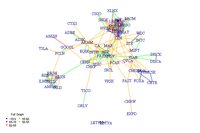
print(join(c('Minimum Spanning Tree based on Pearson Correlation for Nasdaq 100 Components',
'based on daily returns for',format(range(index(ret)), '%d-%b-%Y')), ' '))Minimum Spanning Tree based on Pearson Correlation for Nasdaq 100 Components based on daily returns for 07-Mar-2014 06-Mar-2015
plot.cor(ret, 0.5)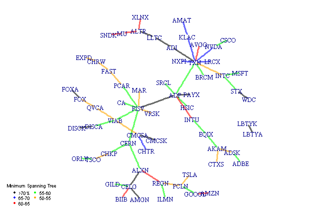
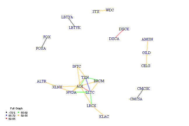
Next let’s get intraday 1 minute historical quotes and visualize correlation based on the last 5 days:
#*****************************************************************
# Load historical intraday quotes
#*****************************************************************
tickers = names(data$prices)

filename = 'data/nasdaq.100.intraday.Rdata'
if(!file.exists(filename)) {
	data1 <- new.env()
	for(ticker in tickers)
		data1[[ticker]] = getSymbol.intraday.google(ticker, 'NASDAQ', 60, '15d')
	save(data1, file=filename)
}

load(file=filename)

#print(bt.start.dates(data1))

bt.prep(data1, align='keep.all', fill.gaps=T)


#*****************************************************************
# Visualize Correlation Matrix
#*****************************************************************
prices = data1$prices

ret = diff(log(prices))
	# there are 391 = 6*60+30+1 entries each day
	# i.e. dim(data1$AAPL['2015:03:03'])
	# last 5 days
	ret = last(ret, 5 * ( 6*60+30+1))

print(join(c('Minimum Spanning Tree based on Pearson Correlation for Nasdaq 100 Components',
'based on 1 minute returns for',format(range(index(ret)), '%d-%b-%Y %H-%M')), ' '))
Minimum Spanning Tree based on Pearson Correlation for Nasdaq 100 Components based on 1 minute returns for 02-Mar-2015 09-30 06-Mar-2015 16-00
plot.cor(ret, 0.5)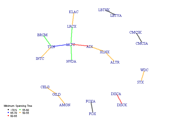
Helper functions:
#*****************************************************************
# Helper Function to Create / Clean Correlation Matrix
#*****************************************************************
clean.cor = function(ret, threshold = 0.5) {
	cor_mat = cor(coredata(ret), use='complete.obs',method='pearson')

	cor_mat[ abs(cor_mat) < threshold] = 0

	keep.index = rowSums(cor_mat != 0) > 1

	cor_mat = cor_mat[keep.index, keep.index]

	cor_mat[ lower.tri(cor_mat, diag=TRUE) ] = 0

	cor_mat
}

#*****************************************************************
# Helper Function to Plot Minimum Spanning Tree
#*****************************************************************
plot.cor = function(ret, threshold = 0.5) {
	cor_mat = clean.cor(ret, threshold)

	transform.fn = function(x) x
	transform.fn = function(x) sqrt(2.0 * ( 1 - x ) )
	transform.fn = function(x) 1 - abs( x )

	dist = transform.fn( cor_mat )
		dist[cor_mat == 0] = 0

	load.packages('igraph')
	graph = graph.adjacency(dist, weighted=TRUE, mode='upper')
	mst = minimum.spanning.tree(graph)

	breaks = c(0,55,60,65,70,100)
	cols = spl('black,blue,red,green,orange')
	labels = 1:5

	factor = cut(E(mst)$weight, breaks = transform.fn(breaks/100), labels = labels)
	for(i in labels)
		E(mst)[ factor == i ]$color = col.add.alpha(cols[i],150)

	set.seed(100)
	par(mar=c(1,1,1,1))
	plot(mst,vertex.size=5, vertex.color=NA, vertex.frame.color=NA, edge.width = 3)

	legend('bottomleft', title='Minimum Spanning Tree', cex=0.75, pch=16, bty='n', ncol=2,
		col=spl('black,blue,red,green,orange'),
		legend=spl('>70%,65-70,60-65,55-60,50-55')
	)

	# full graph
	factor = cut(E(graph)$weight, breaks = transform.fn(breaks/100), labels = labels)
	for(i in labels)
		E(graph)[ factor == i ]$color = col.add.alpha(cols[i],100)

	set.seed(100)
	plot(graph,vertex.size=5, vertex.color=NA, vertex.frame.color=NA, edge.width = 3)

	legend('bottomleft', title='Full Graph', cex=0.75, pch=16, bty='n', ncol=2,
		col=spl('black,blue,red,green,orange'),
		legend=spl('>70%,65-70,60-65,55-60,50-55')
	)
}
(this report was produced on: 2015-03-08)