Logical Invest Universal Investment Strategy (UIS)
02 Dec 2014To install Systematic Investor Toolbox (SIT) please visit About page.
Look at Frank Grossmann’s blog post: The SPY-TLT Universal Investment Strategy (UIS)
The real world is just not a 100% “risk on” or “risk off” world. Most of the time, the best allocation is somewhere in between.
Load historical data for SPY and TLT, and align it, so that dates on both time series match. We also adjust data for stock splits and dividends.
	#*****************************************************************
	# Load historical data
	#*****************************************************************
	library(SIT)
	load.packages('quantmod')
	tickers = spl('SPY,TLT')

	data <- new.env()
	getSymbols(tickers, src = 'yahoo', from = '1970-01-01', env = data, auto.assign = T)
		for(i in ls(data)) data[[i]] = adjustOHLC(data[[i]], use.Adjusted=T)
	bt.prep(data, align='remove.na')
Now we ready to back-test our strategy:
	#*****************************************************************
	# Code Strategies
	#*****************************************************************
	prices = data$prices
	n = ncol(prices)
	month.ends = endpoints(prices, 'months')

	models = list()

	commission = list(cps = 0.01, fixed = 10.0, percentage = 0.0)

	#*****************************************************************
	# Code Strategies, SPY - Buy & Hold
	#*****************************************************************
	data$weight[] = NA
		data$weight$SPY = 1
	models$SPY = bt.run.share(data, clean.signal=T, commission = commission, trade.summary=T, silent=T)


	#*****************************************************************
	# Code Strategies, Equal Weight, re-balanced monthly
	#*****************************************************************
	data$weight[] = NA
		data$weight[month.ends,] = ntop(prices, n)[month.ends,]
	models$equal.weight = bt.run.share(data, clean.signal=F, commission = commission, trade.summary=T, silent=T)


	#*****************************************************************
	# Code Strategies, Top 1 based on 3 month momentum, re-balanced monthly
	#*****************************************************************
	position.score = prices / mlag(prices, 3*21)

	data$weight[] = NA
		data$weight[month.ends,] = ntop(position.score[month.ends,], 1)
	models$top1 = bt.run.share(data, clean.signal=F, commission = commission, trade.summary=T, silent=T)


	#*****************************************************************
	# Code Strategies, Logical Invest Universal Investment Strategy (UIS)
	#*****************************************************************
adaptive.weight <- function(prices, lookback = 80, f=2, index = 1:nrow(prices)) {
	if( len(lookback) == 1 ) lookback = rep(lookback, len(index))
	if( len(f) == 1 ) f = rep(f, len(index))

	ret = prices / mlag(prices) - 1
		ret = coredata(ret)

	allocation = seq(0,100,10)
	allocation = cbind(allocation, 100-allocation)/100

	out = NA * prices
	index = index[index>0]
	for(i in 1:len(index)) {
		if(index[i] < lookback[i]) next

		allocation.ret = ret[(index[i] - lookback[i] + 1) : index[i],] %*% t(allocation)

		allocation.sd = apply(allocation.ret, 2, sd)
		allocation.mean = apply(allocation.ret, 2, mean)
		metric = allocation.mean/(allocation.sd ^ f)

		j = which.max(metric)

		out[index[i],] = allocation[j,]
	}
	out
}

tic(10)
	weight = adaptive.weight(prices, index = month.ends)
toc(10)
Elapsed time is 0.15 seconds
	data$weight[] = NA
		data$weight[month.ends,] = weight[month.ends,]
	models$UIS = bt.run.share(data, clean.signal=F, commission = commission, trade.summary=T, silent=T)


tic(10)
	for(lookback in seq(50,80,5))
		for(f in seq(0.5,3,0.1))
			weight = weight + adaptive.weight(prices, lookback = lookback, f=f, index = month.ends)
toc(10)
Elapsed time is 20.84 seconds
	weight[month.ends,] = weight[month.ends,] / rowSums(weight[month.ends,])


	data$weight[] = NA
		data$weight[month.ends,] = weight[month.ends,]
	models$UISA = bt.run.share(data, clean.signal=F, commission = commission, trade.summary=T, silent=T)


	#*****************************************************************
	# Create Report
	#*****************************************************************
	plotbt(models, plotX = T, log = 'y', LeftMargin = 3, main = NULL)
		mtext('Cumulative Performance', side = 2, line = 1)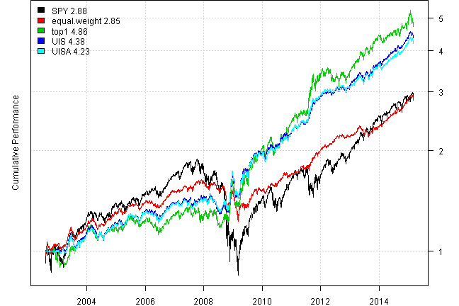
print(plotbt.strategy.sidebyside(models, make.plot=F, return.table=T))| SPY | equal.weight | top1 | UIS | UISA | |
|---|---|---|---|---|---|
| Period | Jul2002 - Mar2015 | Jul2002 - Mar2015 | Jul2002 - Mar2015 | Jul2002 - Mar2015 | Jul2002 - Mar2015 |
| Cagr | 8.74 | 8.65 | 13.35 | 12.42 | 12.1 |
| Sharpe | 0.52 | 0.96 | 0.94 | 1.22 | 1.19 |
| DVR | 0.34 | 0.83 | 0.79 | 1.06 | 1.05 |
| Volatility | 19.78 | 9.11 | 14.52 | 10.06 | 10 |
| MaxDD | -55.19 | -24.91 | -17.08 | -15.81 | -17.17 |
| AvgDD | -1.92 | -1.14 | -2.13 | -1.33 | -1.36 |
| VaR | -1.84 | -0.88 | -1.44 | -0.95 | -0.94 |
| CVaR | -2.98 | -1.3 | -2.03 | -1.44 | -1.44 |
| Exposure | 99.97 | 99.94 | 97.89 | 97.26 | 97.26 |
print(last.trades(models$top1, make.plot=F, return.table=T)) | models$top1 | weight | entry.date | exit.date | nhold | entry.price | exit.price | return |
|---|---|---|---|---|---|---|---|
| SPY | 100 | 2013-07-31 | 2013-08-30 | 30 | 163.78 | 158.87 | -3.00 |
| SPY | 100 | 2013-08-30 | 2013-09-30 | 31 | 158.87 | 163.90 | 3.17 |
| SPY | 100 | 2013-09-30 | 2013-10-31 | 31 | 163.90 | 171.49 | 4.63 |
| SPY | 100 | 2013-10-31 | 2013-11-29 | 29 | 171.49 | 176.57 | 2.96 |
| SPY | 100 | 2013-11-29 | 2013-12-31 | 32 | 176.57 | 181.15 | 2.59 |
| SPY | 100 | 2013-12-31 | 2014-01-31 | 31 | 181.15 | 174.77 | -3.52 |
| TLT | 100 | 2014-01-31 | 2014-02-28 | 28 | 104.95 | 105.50 | 0.52 |
| TLT | 100 | 2014-02-28 | 2014-03-31 | 31 | 105.50 | 106.28 | 0.74 |
| TLT | 100 | 2014-03-31 | 2014-04-30 | 30 | 106.28 | 108.50 | 2.09 |
| SPY | 100 | 2014-04-30 | 2014-05-30 | 30 | 185.52 | 189.82 | 2.32 |
| TLT | 100 | 2014-05-30 | 2014-06-30 | 31 | 111.71 | 111.43 | -0.25 |
| SPY | 100 | 2014-06-30 | 2014-07-31 | 31 | 193.74 | 191.14 | -1.34 |
| SPY | 100 | 2014-07-31 | 2014-08-29 | 29 | 191.14 | 198.68 | 3.94 |
| TLT | 100 | 2014-08-29 | 2014-09-30 | 32 | 117.46 | 114.98 | -2.11 |
| TLT | 100 | 2014-09-30 | 2014-10-31 | 31 | 114.98 | 118.22 | 2.82 |
| TLT | 100 | 2014-10-31 | 2014-11-28 | 28 | 118.22 | 121.73 | 2.97 |
| SPY | 100 | 2014-11-28 | 2014-12-31 | 33 | 206.06 | 205.54 | -0.25 |
| TLT | 100 | 2014-12-31 | 2015-01-30 | 30 | 125.42 | 137.73 | 9.82 |
| TLT | 100 | 2015-01-30 | 2015-02-27 | 28 | 137.73 | 129.28 | -6.14 |
| TLT | 100 | 2015-02-27 | 2015-03-11 | 12 | 129.28 | 127.20 | -1.61 |
	#*****************************************************************
	# Same for 2014
	#*****************************************************************
	models1 = bt.trim(models, dates = '2014')


	#*****************************************************************
	# Create Report
	#*****************************************************************
	plotbt(models1, plotX = T, log = 'y', LeftMargin = 3, main = NULL)
		mtext('Cumulative Performance', side = 2, line = 1)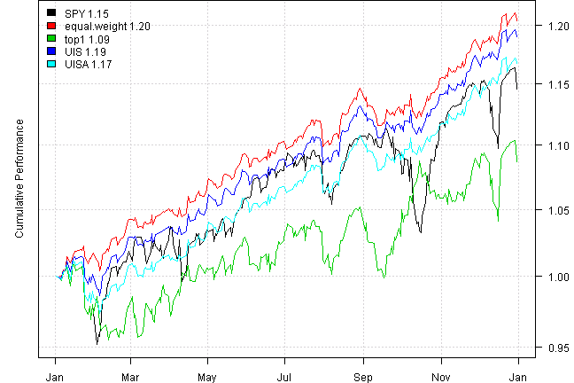
print(plotbt.strategy.sidebyside(models1, make.plot=F, return.table=T))| SPY | equal.weight | top1 | UIS | UISA | |
|---|---|---|---|---|---|
| Period | Jan2014 - Dec2014 | Jan2014 - Dec2014 | Jan2014 - Dec2014 | Jan2014 - Dec2014 | Jan2014 - Dec2014 |
| Cagr | 14.65 | 20.49 | 8.69 | 19.09 | 16.77 |
| Sharpe | 1.18 | 3.25 | 0.74 | 2.83 | 2.39 |
| DVR | 1 | 3.16 | 0.58 | 2.74 | 2.29 |
| Volatility | 11.25 | 5.65 | 10.69 | 6 | 6.19 |
| MaxDD | -7.27 | -2.67 | -5.4 | -2.79 | -3.72 |
| AvgDD | -1.45 | -0.53 | -1.89 | -0.61 | -0.66 |
| VaR | -1.16 | -0.58 | -1.06 | -0.58 | -0.63 |
| CVaR | -1.72 | -0.78 | -1.46 | -0.84 | -0.92 |
| Exposure | 100 | 100 | 100 | 100 | 100 |
	#*****************************************************************
	# Same for last 5 years
	#*****************************************************************
	models1 = bt.trim(models, dates = '2010::')


	#*****************************************************************
	# Create Report
	#*****************************************************************
	plotbt(models1, plotX = T, log = 'y', LeftMargin = 3, main = NULL)
		mtext('Cumulative Performance', side = 2, line = 1)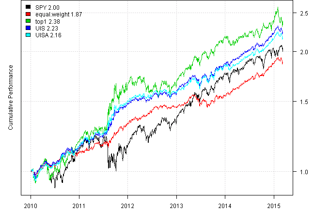
print(plotbt.strategy.sidebyside(models1, make.plot=F, return.table=T))| SPY | equal.weight | top1 | UIS | UISA | |
|---|---|---|---|---|---|
| Period | Jan2010 - Mar2015 | Jan2010 - Mar2015 | Jan2010 - Mar2015 | Jan2010 - Mar2015 | Jan2010 - Mar2015 |
| Cagr | 14.28 | 12.89 | 18.23 | 16.71 | 16.02 |
| Sharpe | 0.94 | 1.76 | 1.22 | 1.92 | 1.79 |
| DVR | 0.88 | 1.72 | 1.19 | 1.88 | 1.76 |
| Volatility | 15.81 | 7.11 | 14.88 | 8.36 | 8.66 |
| MaxDD | -18.61 | -7.14 | -12.03 | -6.48 | -6.78 |
| AvgDD | -1.71 | -0.83 | -2.09 | -0.97 | -1.04 |
| VaR | -1.61 | -0.71 | -1.46 | -0.8 | -0.81 |
| CVaR | -2.39 | -1 | -2.01 | -1.19 | -1.22 |
| Exposure | 100 | 100 | 100 | 100 | 100 |
The idea for this Universal Investment Strategy was to develop a strategy which has an adaptive allocation between 0% and 100% for each ETF depending of the market situation.
The way to calculate the optimum composition is done by calculating which composition had the maximum Sharpe ratio during an optimized look back period (normally 50-80 days). During normal market periods, the maximum Sharpe ratio is not at a 100% SPY or at a 100% TLT allocation, but somewhere in between.
To calculate this maximum Sharpe ratio, I loop through all possible compositions from 0%SPY-100%TLT to 100%SPY-0%TLT and calculate the resulting Sharpe ratio for the look back period.
Sample test of process:
ret = prices / mlag(prices) - 1
	ret = coredata(ret)

i = dates2index(prices, '2014:07:21')
index = (i - 80 + 1) : i

f = 1

allocation = seq(0,100,5)
	allocation = cbind(allocation, 100-allocation)/100

allocation.ret = ret[index,] %*% t(allocation)

allocation.sd = apply(allocation.ret, 2, sd)
allocation.mean = apply(allocation.ret, 2, mean)

out = rbind(t(allocation), allocation.mean/(allocation.sd ^ f), sqrt(252)*allocation.sd, 252*allocation.mean)
	rownames(out) = spl('SPY,TLT,Sharpe,Volatility,Return')
	colnames(out) = out['SPY',]
print( to.percent(out[,which.max(out['Sharpe',]),drop=F]) )| 0.55 | |
|---|---|
| SPY | 55.00% |
| TLT | 45.00% |
| Sharpe | 27.93% |
| Volatility | 4.75% |
| Return | 21.07% |
out = round(100*out,1)


plot(out['SPY',],out['Sharpe',], type='l', col='black',
	las=1, ylim=c(0,30), xlab='SPY Allocation', ylab='')
	lines(out['SPY',],out['Volatility',], type='l', col='orange')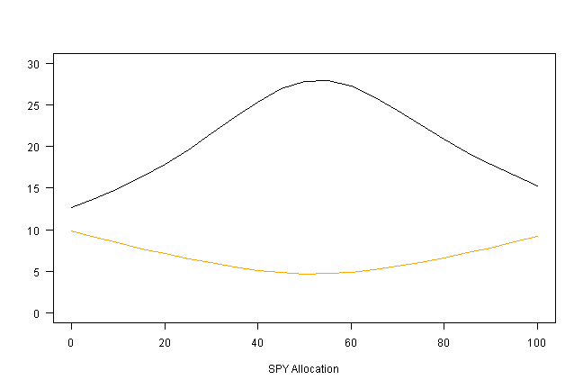
print(out)| 0 | 0.05 | 0.1 | 0.15 | 0.2 | 0.25 | 0.3 | 0.35 | 0.4 | 0.45 | 0.5 | 0.55 | 0.6 | 0.65 | 0.7 | 0.75 | 0.8 | 0.85 | 0.9 | 0.95 | 1 | |
|---|---|---|---|---|---|---|---|---|---|---|---|---|---|---|---|---|---|---|---|---|---|
| SPY | 0 | 5 | 10 | 15 | 20 | 25 | 30 | 35 | 40 | 45 | 50 | 55 | 60 | 65 | 70 | 75 | 80 | 85 | 90 | 95 | 100 |
| TLT | 100 | 95 | 90 | 85 | 80 | 75 | 70 | 65 | 60 | 55 | 50 | 45 | 40 | 35 | 30 | 25 | 20 | 15 | 10 | 5 | 0 |
| Sharpe | 12.6 | 13.7 | 14.9 | 16.3 | 17.8 | 19.6 | 21.5 | 23.5 | 25.3 | 26.9 | 27.8 | 27.9 | 27.3 | 26 | 24.3 | 22.6 | 20.9 | 19.2 | 17.8 | 16.5 | 15.3 |
| Volatility | 9.8 | 9.1 | 8.4 | 7.7 | 7.1 | 6.5 | 6 | 5.5 | 5.1 | 4.9 | 4.7 | 4.8 | 4.9 | 5.2 | 5.6 | 6 | 6.6 | 7.2 | 7.8 | 8.5 | 9.2 |
| Return | 19.6 | 19.7 | 19.8 | 20 | 20.1 | 20.2 | 20.4 | 20.5 | 20.7 | 20.8 | 20.9 | 21.1 | 21.2 | 21.3 | 21.5 | 21.6 | 21.8 | 21.9 | 22 | 22.2 | 22.3 |
(this report was produced on: 2015-03-12)