Leadership Details
16 Apr 2015To install Systematic Investor Toolbox (SIT) please visit About page.
Let’s continue with Run Leadership Rcpp post and look at results in more details
First, let’s load historical prices for S&P 500:
#*****************************************************************
# Load historical end of day data
#*****************************************************************
library(SIT)
load.packages('quantmod')

filename = 'big.test.Rdata'

if(!file.exists(filename)) {
  tickers = nasdaq.100.components()
  tickers = sp500.components()$tickers

  data = env()
  getSymbols.extra(tickers, src = 'yahoo', from = '1970-01-01', env = data, auto.assign = T)

	rm.index = which(sapply(ls(data), function(i) is.null(data[[i]])))
	if(any(rm.index)) env.del(names(rm.index), data)

  for(i in ls(data)) data[[i]] = adjustOHLC(data[[i]], use.Adjusted=T)
  #print(bt.start.dates(data))

  bt.prep(data, align='keep.all', dates='2000::', fill.gaps=T)

  # remove ones with little history
  prices = data$prices
  bt.prep.remove.symbols(data, which(
   	count(prices, side = 2) < 3*252 | is.na(last(prices))
  ))

  # show the ones removed
  print(setdiff(tickers,names(data$prices)))

  prices = data$prices
  save(prices, file=filename)
}

load(file=filename)

#*****************************************************************
# Helper functions
#*****************************************************************
# lead - lag sample function
rtest = function(ret, nwindow) {
	nlag = floor(nwindow/2)
	n = ncol(ret)
	nperiod = nrow(ret)
	out = array(0, c(n,n,nperiod))
	index = !lower.tri(out[,,1])

	for(i in nwindow:nperiod) {
		temp = coredata(ret[(i-nwindow+1):i,])
		temp.out = matrix(0, n,n)

		for (c1 in 2:n) {
			data1 = temp[,c1]
			c2.index = 1:(c1-1)
			data2 = temp[,c2.index,drop=F]

			# if c1.cor : c2 -> c1 i.e. cor(data1[(lag+1):nwindow], data2[1:(nwindow-lag),])
			c1.cor = rep(0,ncol(data2))
			for (lag in 0:nlag) {
				cor.temp = cor(data1[(lag+1):nwindow], data2[1:(nwindow-lag),])
				c1.cor = c1.cor + pmax(cor.temp, 0)
			}
			c1.cor = c1.cor / (nlag + 1)

			# if c2.cor : c1 -> c2 i.e. cor(data1[1:(nwindow-lag)], data2[(lag+1):nwindow,])
			c2.cor = rep(0,ncol(data2))
			for (lag in 1:nlag) {
				cor.temp = cor(data1[1:(nwindow-lag)], data2[(lag+1):nwindow,])
				c2.cor = c2.cor + pmax(cor.temp, 0)
			}
			c2.cor = c2.cor / nlag

			# if c1.cor >= c2.cor hence c2 -> c1 i.e. cor(data1[(lag+1):nwindow], data2[1:(nwindow-lag),])
			index = c1.cor >= c2.cor
			if(any(index))
				temp.out[c2.index[index], c1] = c1.cor[index]

			# if c2.cor >= c1.cor hence c1 -> c2 i.e. cor(data1[1:(nwindow-lag)], data2[(lag+1):nwindow,])
			index = !index
			if(any(index))
				temp.out[c1, c2.index[index]] = c2.cor[index]
		}
		out[,,i] = temp.out
	}
	out
}


# lead - lag sample function
rtest.one = function(ret, nwindow, c1.name, c2.name) {
	c1 = which(colnames(ret) == c1.name)
	c2 = which(colnames(ret) == c2.name)
	if(c1 < c2) { # switch
		temp = c2; c2 = c1; c1 = temp
		temp = c2.name; c2.name = c1.name; c1.name = temp
	}

	nlag = floor(nwindow/2)
	n = ncol(ret)
	nperiod = nrow(ret)
	out = array(NA, c(n,n,nperiod))
	index = !lower.tri(out[,,1])

	i = nperiod

		temp = coredata(ret[(i-nwindow+1):i,])
		temp.out = matrix(NA, n,n)

			data1 = temp[,c1]
			data2 = temp[,c2,drop=F]

			c1.cor = c()
			for (lag in 0:nlag) {
				cor.temp = cor(data1[(lag+1):nwindow], data2[1:(nwindow-lag),])
				c1.cor = c(c1.cor, cor.temp)
			}

			c2.cor = c()
			for (lag in 1:nlag) {
				cor.temp = cor(data1[1:(nwindow-lag)], data2[(lag+1):nwindow,])
				c2.cor = c(c2.cor, cor.temp)
			}


			c1.cor.mean = sum(pmax(c1.cor,0)) / (nlag + 1)
			c2.cor.mean = sum(pmax(c2.cor,0)) / nlag
			# if c1.cor >= c2.cor hence c2 -> c1 i.e. cor(data1[(lag+1):nwindow], data2[1:(nwindow-lag),])
			# if c2.cor >= c1.cor hence c1 -> c2 i.e. cor(data1[1:(nwindow-lag)], data2[(lag+1):nwindow,])
			relationship = iif(c1.cor.mean >= c2.cor.mean, 'c2 -> c1', 'c1 -> c2')

		list(
			c1 = c1, c2 = c2, c1.name = c1.name, c2.name = c2.name,
			x = -nlag:nlag,
			y = c(c2.cor, c1.cor),
			c1.cor = to.nice(c1.cor.mean),
			c2.cor = to.nice(c2.cor.mean),
			relationship = relationship,
			c1.ret = ret[(i-nwindow+1):i,c1],
			c2.ret = ret[(i-nwindow+1):i,c2]

		)
}
# make plot
rtest.visualize = function(out) {
	par(mar=c(5,4,4,5))
	plot(out$x, out$y, type = "n", xlab='Lag', ylab='Correlation', las=1,
		main = paste('c2 =', out$c2.name, out$c2.cor, 'vs c1 =', out$c1.name, out$c1.cor,
		'\n', out$relationship)
	)
	col1 = col.add.alpha('blue',100)
	polygon(c(first(out$x), out$x, last(out$x)), c(0, pmax(out$y,0), 0), col=col1, border=col1)
	col1 = col.add.alpha('gray',200)
	polygon(c(first(out$x), out$x, last(out$x)), c(0, pmin(out$y,0), 0), col=col1, border=col1)
	abline(h=0, v=0)
	lines(out$x, out$y, col='red')
	lines(out$x, out$y, type='b', pch='+', col='red')
}
rtest.visualize.relationship = function(out) {
	ylim = range(c(cumprod(1 + out$c1.ret), cumprod(1 + out$c2.ret)))
	plota(cumprod(1 + out$c1.ret), type='l', ylim = ylim, col='black')
		plota.lines(cumprod(1 + out$c2.ret), col='blue')
		plota.legend(paste('c1', out$c1.name, ',c2', out$c2.name, ',', out$relationship), 'black,blue, red')
}


#*****************************************************************
# Run Lead Lag Correlation
#*****************************************************************
prices = prices[,]

n = ncol(prices)
nperiod = nrow(prices)
ret = prices / mlag(prices) - 1

index =  (nperiod-20):nperiod
ret = ret[index,]
nperiod = nrow(ret)
nwindow = 15

#*****************************************************************
# Run Lead Lag Correlation
#*****************************************************************
# make sure to install [Rtools on windows](http://cran.r-project.org/bin/windows/Rtools/)
load.packages('Rcpp')
load.packages('RcppParallel')

# load Rcpp functions
sourceCpp('lead.lag.correlation.cpp')

c.cor = cp_run_leadership_smart(ret, nwindow, T)

# remove zero entries
clean.adj = function(adj.mat, threshold = 0.5) {
	adj.mat[ abs(adj.mat) < threshold] = 0
	keep.index = (rowSums(adj.mat != 0) >= 1) | (colSums(adj.mat != 0) >= 1)
	adj.mat = adj.mat[keep.index, keep.index]
	adj.mat
}

adj.mat = c.cor[,,nperiod-1]
	rownames(adj.mat) = colnames(adj.mat) = colnames(prices)
	adj.mat = clean.adj(adj.mat, 0.38)

temp = adj.mat
	temp[temp == 0] = NA
print(to.percent(temp))| AIG | APA | ED | NEM | PPL | PVH | RL | STT | XL | |
|---|---|---|---|---|---|---|---|---|---|
| AIG | |||||||||
| APA | |||||||||
| ED | 38.18% | ||||||||
| NEM | |||||||||
| PPL | |||||||||
| PVH | 41.76% | ||||||||
| RL | 42.19% | 38.71% | |||||||
| STT | 38.28% | ||||||||
| XL | 38.30% |
# examine some pairs
out = rtest.one(ret, nwindow, 'AIG', 'PVH')
	rtest(ret[,c(out$c2,out$c1)], nwindow)[,,nperiod]
[,1] [,2] [1,] 0.0000000 0 [2,] 0.3668593 0
rtest.visualize(out)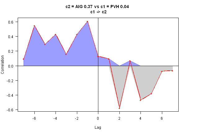
rtest.visualize.relationship(out)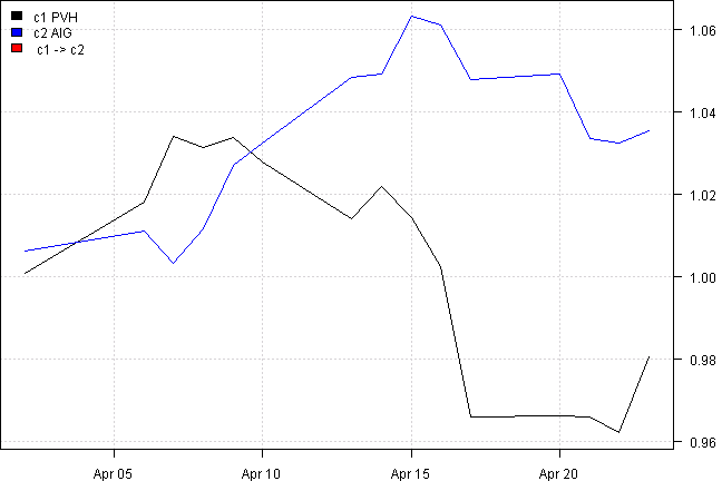
out = rtest.one(ret, nwindow, 'XL', 'RL')
	rtest(ret[,c(out$c2,out$c1)], nwindow)[,,nperiod]
[,1] [,2] [1,] 0 0.2261738 [2,] 0 0.0000000
rtest.visualize(out)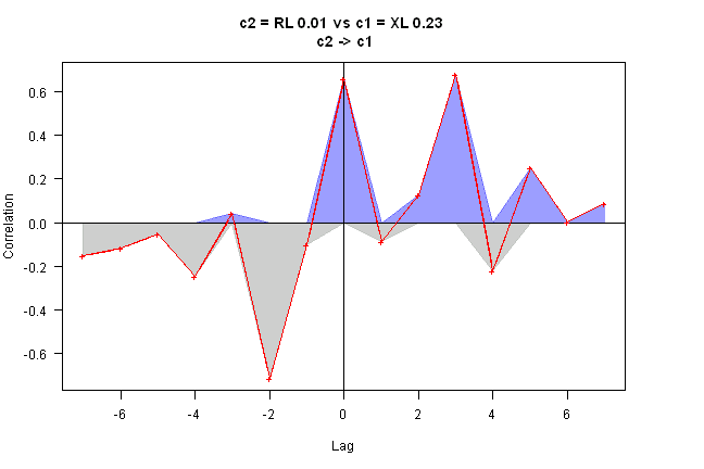
rtest.visualize.relationship(out)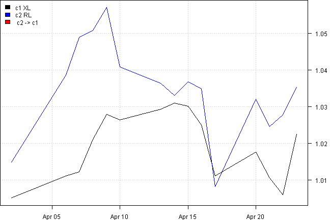
out = rtest.one(ret, nwindow, 'APA', 'XL')
	rtest(ret[,c(out$c2,out$c1)], nwindow)[,,nperiod]
[,1] [,2] [1,] 0.0000000 0 [2,] 0.3136286 0
rtest.visualize(out)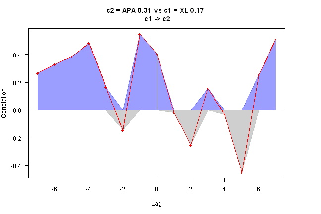
rtest.visualize.relationship(out)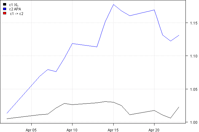
# adj.mat(row,col) is mapped to
#
# |from |to  |value            |
# |:----|:---|:----------------|
# |row  |col |adj.mat(row,col) |

load.packages('igraph')
g  = graph.adjacency(adj.mat,weighted=TRUE)
get.data.frame(g)
from to weight 1 ED PPL 0.3817913 2 PVH AIG 0.4175742 3 RL AIG 0.4219342 4 RL XL 0.3870656 5 STT NEM 0.3828356 6 XL APA 0.3830476
print(g)IGRAPH DNW- 9 6 -- + attr: name (v/c), weight (e/n)
(this report was produced on: 2015-04-24)