Historical Country Returns
26 Mar 2016To install Systematic Investor Toolbox (SIT) please visit About page.
There are not many sources of historical country returns. You might use Country ETFs, but usually they do not have a long history. Let’s compare the historical country returns data from:
Load historical country returns from AQR data library
#*****************************************************************
# Read historical data from AQR library
# [Betting Against Beta: Equity Factors, Monthly](https://www.aqr.com/library/data-sets/betting-against-beta-equity-factors-monthly)
#******************************************************************
library(readxl)
library(SIT)
library(quantmod)

data = env()
data.set = 'betting-against-beta-equity-factors'

# monthly market returns in excess of t-bills
data$market.excess = load.aqr.data(data.set, 'monthly', 'MKT')

#monthly U.S. Treasury bill rates.
data$risk.free = load.aqr.data(data.set, 'monthly', 'RF', last.col2extract = 2)

# total market return
aqr.market = data$market.excess + as.vector(data$risk.free)

# check data starting dates
start.dates = function(data) {
	sapply(colnames(data), function(n)
		format( index(na.omit(data[,n])[1]), '%Y %b %d')
	)
}

print( sort(start.dates(aqr.market)) )| USA | CAN | AUS | AUT | BEL | CHE | DEU | DNK | ESP | FIN | FRA | GBR | HKG | IRL | ITA | JPN | NLD | NOR | NZL | SGP | SWE | PRT | GRC | ISR |
|---|---|---|---|---|---|---|---|---|---|---|---|---|---|---|---|---|---|---|---|---|---|---|---|
| 1926 Jul 31 | 1981 Feb 28 | 1985 Nov 30 | 1986 Jan 31 | 1986 Jan 31 | 1986 Jan 31 | 1986 Jan 31 | 1986 Jan 31 | 1986 Jan 31 | 1986 Jan 31 | 1986 Jan 31 | 1986 Jan 31 | 1986 Jan 31 | 1986 Jan 31 | 1986 Jan 31 | 1986 Jan 31 | 1986 Jan 31 | 1986 Jan 31 | 1986 Jan 31 | 1986 Jan 31 | 1986 Jan 31 | 1988 Feb 29 | 1988 Sep 30 | 1994 Dec 31 |
Load historical country returns from Kenneth R. French - Data Library
#*****************************************************************
# Read historical data from Kenneth R. French - Data Library
# [U.S. Research Returns Data](http://mba.tuck.dartmouth.edu/pages/faculty/ken.french/ftp/F-F_Research_Data_Factors.zip)
# [International Research Returns Data](http://mba.tuck.dartmouth.edu/pages/faculty/ken.french/ftp/F-F_International_Countries.zip)
#******************************************************************
data.set = 'F-F_Research_Data_Factors'
data = get.fama.french.data(data.set, 'months')
	US.Mkt.RF = data[[1]]$Mkt.RF
	US.RF = data[[1]]$RF

data.set = 'F-F_International_Countries'
data = get.fama.french.data(data.set, 'months', file.suffix='')

temp = env()
for(n in ls(data))
	temp[[n]] = make.stock.xts(data[[n]][[1]]$.Mkt)
temp$US = make.stock.xts(US.Mkt.RF + US.RF)

bt.prep(temp, align='keep.all', fill.gaps = F)
	ff.market = temp$prices

print( sort(start.dates(ff.market)) )| US | Austrlia | Belgium | France | Germany | HongKong | Italy | Japan | Nethrlnd | Norway | Singapor | Spain | Sweden | Swtzrlnd | UK | Canada | Austria | Finland | NewZland | Denmark | Ireland | Malaysia |
|---|---|---|---|---|---|---|---|---|---|---|---|---|---|---|---|---|---|---|---|---|---|
| 1926 Jul 01 | 1975 Jan 01 | 1975 Jan 01 | 1975 Jan 01 | 1975 Jan 01 | 1975 Jan 01 | 1975 Jan 01 | 1975 Jan 01 | 1975 Jan 01 | 1975 Jan 01 | 1975 Jan 01 | 1975 Jan 01 | 1975 Jan 01 | 1975 Jan 01 | 1975 Jan 01 | 1977 Jan 01 | 1987 Jan 01 | 1988 Jan 01 | 1988 Jan 01 | 1989 Jan 01 | 1991 Jan 01 | 1994 Jan 01 |
Examine historical country returns side by side
#*****************************************************************
# Compare data: different universe => different returns
#******************************************************************
# convert data into same monthly format
yyyymm = function(x) make.xts( coredata(x), as.Date(ISOdate(date.year(index(x)),date.month(index(x)),1)))
	aqr.market = 100*yyyymm(aqr.market)
	ff.market = yyyymm(ff.market)

# map country codes between AQR and FF
codes = country.code()
aqr.map = codes[,'name']
	names(aqr.map) = codes[,'code3']

ff.map = names(ff.market)
	names(ff.map) = ff.map
	# add custom mapping
	ff.map['Austrlia'] = 'Australia'
	ff.map['HongKong'] = "Hong Kong, Special Administrative Region of China"
	ff.map['Swtzrlnd'] = 'Switzerland'
	ff.map['Singapor'] = 'Singapore'
	ff.map['NewZland'] = "New Zealand"
	ff.map['UK'] = "United Kingdom"
	ff.map['US'] = "United States of America"
	ff.map['Nethrlnd'] = "Netherlands"
	ff.map['Nethrlnd'] = "Netherlands"

# print differences
setdiff( aqr.map[names(aqr.market)] , ff.map[names(ff.market)] )
[1] “Greece” “Israel” “Portugal”
setdiff( ff.map[names(ff.market)] , aqr.map[names(aqr.market)] )[1] “Malaysia”
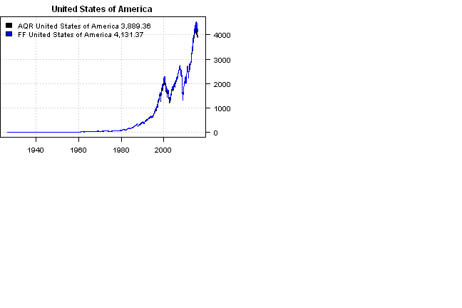
# plot side by side
layout(matrix(1:4,2,2))
common = intersect( aqr.map[names(aqr.market)] , ff.map[names(ff.market)] )
for(n in common) {
	aqr.index = which(aqr.map[names(aqr.market)]==n)
	ff.index = which(ff.map[names(ff.market)]==n)

	temp = merge(na.omit(aqr.market[,aqr.index]), na.omit(ff.market[,ff.index]))
		temp = na.omit(temp)
	temp = bt.apply.matrix(1+temp/100,cumprod)

	plota(temp[,1], col='black', type='l', main=n, ylim = range(temp))
		plota.lines(temp[,2], col='blue', type='l')

	plota.legend(paste(spl('AQR,FF'), n),'black,blue',as.list(temp))
} 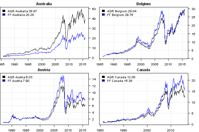
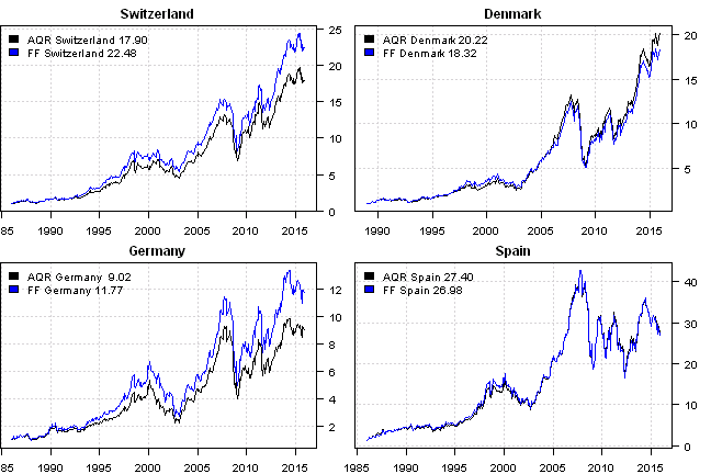
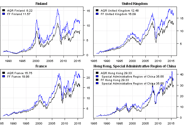
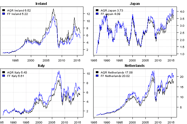
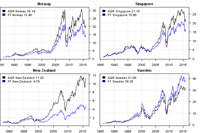
I guess the point is:
- to be aware of different index construction methods and
- do not accept blindly that returns will be identical across different providers
In the end, if you making an allocation decisions based on historical returns, it is best to test robustness of you strategy on different indexes.
Next let’s see how country ETFs, correspond to these historical country returns. For your convenience, the 2016-03-26-Historical-Country-Returns post source code.