Execution Prices
03 Nov 2014To install Systematic Investor Toolbox (SIT) please visit About page.
Load Historical Prices from Yahoo Finance:
	#*****************************************************************
	# Load historical data
	#******************************************************************
	library(SIT)
	load.packages('quantmod')
	tickers = spl('SPY,XLY,XLP,XLE,XLF,XLV,XLI,XLB,XLK,XLU')

	data <- new.env()
	getSymbols(tickers, src = 'yahoo', from = '1970-01-01', env = data, auto.assign = T)
		for(i in ls(data)) data[[i]] = adjustOHLC(data[[i]], use.Adjusted=T)
	bt.prep(data, align='remove.na')
Look at strategies that execute at Open,Close,High,Low:
	#*****************************************************************
	# Code Strategies
	#******************************************************************
	prices = data$prices
	n = len(tickers)

	# find month ends
	month.ends = endpoints(prices, 'months')
		month.ends = month.ends[month.ends > 0]

	models = list()

	#*****************************************************************
	# Code Strategies
	#******************************************************************
	dates = '2001::'

	# Rank on 6 month return
	position.score = prices / mlag(prices, 126)

	frequency = month.ends
	# Select Top 4 funds
	weight = ntop(position.score, 4)

	#*****************************************************************
	# Code Strategies, please note that there is only one price per day
	# so all transactions happen at selected price
	# i.e. below both buys and sells take place at selected price
	#******************************************************************
	for(name in spl('Cl,Op,Hi,Lo')) {
		fun = match.fun(name)

		exec.prices = bt.apply(data, fun)

		data$weight[] = NA
			data$execution.price[] = NA
		  	data$execution.price[frequency,] = exec.prices[frequency,]
		  	data$weight[frequency,] = weight[frequency,]
		models[[name]] = bt.run.share(data, trade.summary=T, dates=dates, silent=T, clean.signal=F)
	}
Look at strategy that Buys Low and Sells High:
	#*****************************************************************
	# Code Strategies
	#******************************************************************
	low.prices = bt.apply(data, Lo)
	high.prices = bt.apply(data, Hi)

	# buy at low price
	execution.price = low.prices[frequency,]

	# sell(i.e. weight=0) at high price
	index = (weight[frequency,])==0
	execution.price[index] = coredata(high.prices[frequency,])[index]

	data$weight[] = NA
		data$execution.price[] = NA
	  	data$execution.price[frequency,] = execution.price
	  	data$weight[frequency,] = weight[frequency,]
	models$Buy.Low.Sell.High = bt.run.share(data, trade.summary=T, dates=dates, silent=T, clean.signal=F)
Look at strategy that Buys High and Sells Low:
	#*****************************************************************
	# Code Strategies
	#******************************************************************
	low.prices = bt.apply(data, Lo)
	high.prices = bt.apply(data, Hi)

	# buy at high price
	execution.price = high.prices[frequency,]

	# sell(i.e. weight=0) at low price
	index = (weight[frequency,])==0
	execution.price[index] = coredata(low.prices[frequency,])[index]

	data$weight[] = NA
		data$execution.price[] = NA
	  	data$execution.price[frequency,] = execution.price
	  	data$weight[frequency,] = weight[frequency,]
	models$Buy.High.Sell.Low = bt.run.share(data, trade.summary=T, dates=dates, silent=T, clean.signal=F)
Create Report:
	#*****************************************************************
	# Create Report
	#******************************************************************
	#strategy.performance.snapshoot(models, T)
	plotbt(models, plotX = T, log = 'y', LeftMargin = 3, main = NULL)
		mtext('Cumulative Performance', side = 2, line = 1)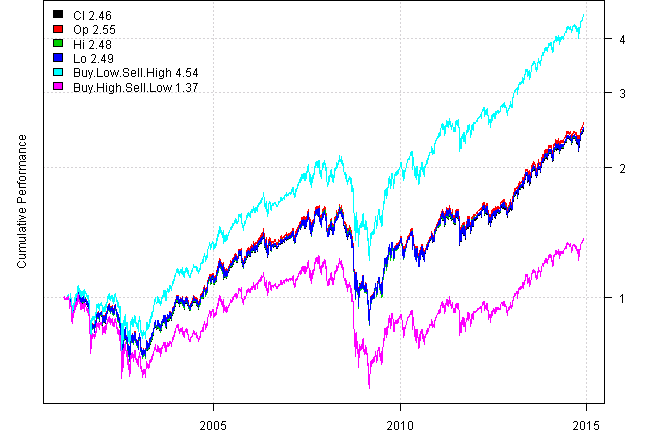
print(plotbt.strategy.sidebyside(models, make.plot=F, return.table=T))| Cl | Op | Hi | Lo | Buy.Low.Sell.High | Buy.High.Sell.Low | |
|---|---|---|---|---|---|---|
| Period | Jan2001 - Dec2014 | Jan2001 - Dec2014 | Jan2001 - Dec2014 | Jan2001 - Dec2014 | Jan2001 - Dec2014 | Jan2001 - Dec2014 |
| Cagr | 6.68 | 6.94 | 6.75 | 6.76 | 11.47 | 2.29 |
| Sharpe | 0.44 | 0.46 | 0.44 | 0.44 | 0.68 | 0.21 |
| DVR | 0.33 | 0.34 | 0.33 | 0.33 | 0.57 | 0.05 |
| Volatility | 18.45 | 18.44 | 18.73 | 18.85 | 18.69 | 18.62 |
| MaxDD | -46.34 | -47.12 | -46.93 | -46.38 | -42.87 | -50.89 |
| AvgDD | -2.74 | -2.65 | -2.74 | -2.71 | -2.31 | -4.19 |
| VaR | -1.9 | -1.86 | -1.91 | -1.91 | -1.85 | -1.91 |
| CVaR | -2.74 | -2.73 | -2.83 | -2.72 | -2.68 | -2.84 |
| Exposure | 99.97 | 99.97 | 99.97 | 99.97 | 99.97 | 99.97 |
Next let’s run same test for a different universe:
bt.execution.price.high.low.test('SPY,EEM,EFA,TLT,IWM,QQQ,GLD', n.top=3)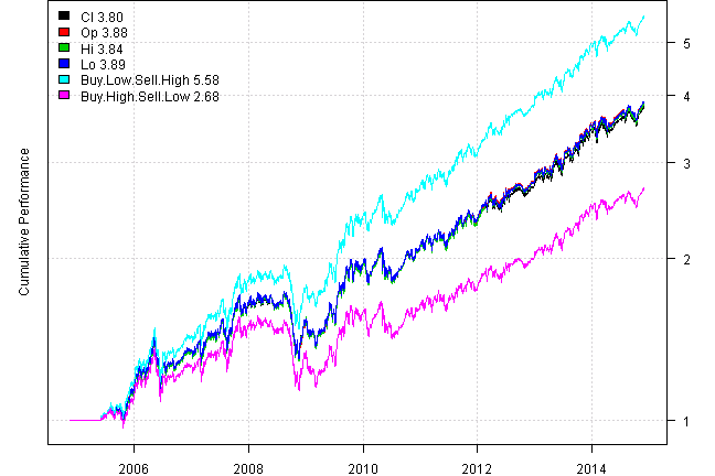
Strategy Performance:
| Cl | Op | Hi | Lo | Buy.Low.Sell.High | Buy.High.Sell.Low | |
|---|---|---|---|---|---|---|
| Period | Nov2004 - Dec2014 | Nov2004 - Dec2014 | Nov2004 - Dec2014 | Nov2004 - Dec2014 | Nov2004 - Dec2014 | Nov2004 - Dec2014 |
| Cagr | 14.21 | 14.45 | 14.33 | 14.46 | 18.66 | 10.32 |
| Sharpe | 0.95 | 0.97 | 0.95 | 0.95 | 1.19 | 0.72 |
| DVR | 0.88 | 0.89 | 0.87 | 0.87 | 1.1 | 0.64 |
| Volatility | 15.19 | 15.13 | 15.42 | 15.55 | 15.42 | 15.33 |
| MaxDD | -24.49 | -25.64 | -25.01 | -24.88 | -23.85 | -27.19 |
| AvgDD | -2.39 | -2.39 | -2.36 | -2.38 | -2.15 | -2.65 |
| VaR | -1.56 | -1.59 | -1.66 | -1.61 | -1.55 | -1.67 |
| CVaR | -2.29 | -2.27 | -2.34 | -2.26 | -2.24 | -2.34 |
| Exposure | 94.74 | 94.74 | 94.74 | 94.74 | 94.74 | 94.74 |
Monthly Results for Cl :
| Jan | Feb | Mar | Apr | May | Jun | Jul | Aug | Sep | Oct | Nov | Dec | Year | MaxDD | |
|---|---|---|---|---|---|---|---|---|---|---|---|---|---|---|
| 2004 | 0.0 | 0.0 | 0.0 | |||||||||||
| 2005 | 0.0 | 0.0 | 0.0 | 0.0 | 0.0 | 2.1 | 2.7 | -0.7 | 1.7 | -3.4 | 5.9 | 5.5 | 14.2 | -7.0 |
| 2006 | 10.0 | -1.9 | 3.3 | 6.3 | -5.4 | -1.5 | 0.4 | 1.1 | -0.5 | 2.6 | 2.6 | 0.3 | 17.5 | -20.6 |
| 2007 | 1.0 | -1.7 | 3.1 | 3.2 | 1.7 | 0.6 | -0.6 | 1.1 | 7.4 | 8.6 | -5.4 | 1.5 | 21.8 | -12.7 |
| 2008 | 1.3 | 2.3 | -2.5 | 0.8 | -0.2 | -1.0 | 0.5 | 2.6 | -7.3 | -13.0 | 5.0 | 7.5 | -5.6 | -24.5 |
| 2009 | -5.7 | -3.6 | 3.9 | 0.9 | 9.8 | -1.5 | 9.5 | 1.6 | 6.5 | -4.1 | 6.0 | 0.4 | 24.7 | -11.2 |
| 2010 | -6.0 | 3.7 | 4.5 | 4.6 | -7.6 | -2.6 | 0.2 | 3.6 | 4.7 | 0.7 | -0.8 | 4.8 | 9.0 | -13.6 |
| 2011 | -0.5 | 4.1 | 0.7 | 2.8 | -1.6 | -1.8 | 1.3 | 4.2 | -0.8 | 4.1 | 0.3 | -2.6 | 10.6 | -8.1 |
| 2012 | 6.5 | 0.3 | 3.6 | -1.1 | -1.3 | 4.2 | 0.2 | 2.1 | 0.3 | -1.8 | 1.2 | 2.9 | 18.1 | -6.2 |
| 2013 | 3.2 | -0.9 | 1.7 | 2.2 | 1.1 | -1.5 | 6.3 | -2.2 | 4.8 | 3.5 | 3.5 | 2.4 | 26.5 | -6.6 |
| 2014 | -3.3 | 4.8 | -0.9 | -1.1 | 3.3 | 1.6 | -0.6 | 3.9 | -3.5 | 2.6 | 3.4 | -0.4 | 9.8 | -6.6 |
| Avg | 0.7 | 0.7 | 1.7 | 1.9 | 0.0 | -0.1 | 2.0 | 1.7 | 1.3 | 0.0 | 2.2 | 2.0 | 13.3 | -10.6 |
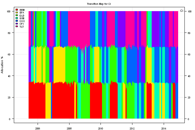
Please note that I added transition chart and monthly performance in the bt.execution.price.high.low.test function.
There seems to be no difference if execution is consistent at Open, Low, High, or Close prices. We can only see a difference where Buy and Sell execution prices differ. For example, buying Low and selling High strategy does better than average strategy and correspondingly buying High and selling Low strategy does worse than average strategy.
(this report was produced on: 2014-12-07)