Conditional Channel Breakout
06 Mar 2015To install Systematic Investor Toolbox (SIT) please visit About page.
David Varadi discussed another interesting concept in the Conditional Percentile Channels post.
Let’s revisit the Channel Breakout - Second Attempt post and use conditional qunatile function developed in the Run Channel in Rcpp post.
Below I will try to adapt a code from David’s post:
#*****************************************************************
# Load historical data
#*****************************************************************
library(SIT)
load.packages('quantmod')

# load saved Proxies Raw Data, data.proxy.raw, to extend DBC and SHY
# please see http://systematicinvestor.github.io/Data-Proxy/ for more details
load('data/data.proxy.raw.Rdata')

tickers = '
LQD + VWESX
DBC + CRB
VTI +VTSMX # (or SPY)
ICF + VGSIX # (or IYR)
CASH = SHY + TB3Y
'

data <- new.env()
getSymbols.extra(tickers, src = 'yahoo', from = '1970-01-01', env = data, raw.data = data.proxy.raw, set.symbolnames = T, auto.assign = T)
for(i in data$symbolnames) data[[i]] = adjustOHLC(data[[i]], use.Adjusted=T)

#print(bt.start.dates(data))
bt.prep(data, align='remove.na', fill.gaps = T)

#*****************************************************************
# Setup
#*****************************************************************
data$universe = data$prices > 0
  # do not allocate to CASH, or BENCH
  data$universe$CASH = NA

prices = data$prices * data$universe
  n = ncol(prices)
  nperiods = nrow(prices)


frequency = 'months'
# find period ends, can be 'weeks', 'months', 'quarters', 'years'
period.ends = endpoints(prices, frequency)
  period.ends = period.ends[period.ends > 0]

models = list()

commission = list(cps = 0.01, fixed = 10.0, percentage = 0.0)

# lag prices by 1 day
#prices = mlag(prices)

#*****************************************************************
# Equal Weight each re-balancing period
#******************************************************************
data$weight[] = NA
  data$weight[period.ends,] = ntop(prices[period.ends,], n)
models$ew = bt.run.share(data, clean.signal=F, commission = commission, trade.summary=T, silent=T)


#*****************************************************************
# Risk Parity each re-balancing period
#******************************************************************
ret = diff(log(prices))
hist.vol = bt.apply.matrix(ret, runSD, n = 20)

# risk-parity
weight = 1 / hist.vol
rp.weight = weight / rowSums(weight, na.rm=T)

data$weight[] = NA
  data$weight[period.ends,] = rp.weight[period.ends,]
models$rp = bt.run.share(data, clean.signal=F, commission = commission, trade.summary=T, silent=T)


#*****************************************************************
# Strategy:
#
# 1) Use 60,120,180, 252-day percentile channels
# - corresponding to 3,6,9 and 12 months in the momentum literature-
# (4 separate systems) with a .75 long entry and .25 exit threshold with
# long triggered above .75 and holding through until exiting below .25
# (just like in the previous post) - no shorts!!!
#
# 2) If the indicator shows that you should be in cash, hold SHY
#
# 3) Use 20-day historical volatility for risk parity position-sizing
# among active assets (no leverage is used). This is 1/volatility (asset A)
# divided by the sum of 1/volatility for all assets to determine the position size.
#******************************************************************

# load conditional qunatile function developed in the [Run Channel in Rcpp](/Run-Channel-Rcpp) post
load.packages('Rcpp')
# you can download `channel.cpp` file at [channel.cpp](/public/doc/channel.cpp)
sourceCpp('channel.cpp')

allocation = 0 * ifna(prices, 0)
for(lookback.len in c(60,120,180, 252)) {
  high.channel = NA * prices
  low.channel = NA * prices
  for(i in 1:ncol(prices)) {
    temp = run_quantile_weight(prices[,i], lookback.len, 0.25, 0.75)
    low.channel[,i] = temp[,1]
    high.channel[,i] = temp[,2]
  }

  signal = iif(cross.up(prices, high.channel), 1, iif(cross.dn(prices, low.channel), -1, NA))
  allocation = allocation + ifna( bt.apply.matrix(signal, ifna.prev), 0)
}

# (A) Channel score
allocation = ifna(allocation / 4, 0)

# equal-weight
weight = abs(allocation) / rowSums(abs(allocation))
	weight[allocation < 0] = 0
weight$CASH = 1 - rowSums(weight, na.rm=T)

data$weight[] = NA
  data$weight[period.ends,] = weight[period.ends,]
models$channel.ew = bt.run.share(data, clean.signal=F, commission = commission, trade.summary=T, silent=T)


# risk-parity: (C)
weight = allocation * 1 / hist.vol
weight = abs(weight) / rowSums(abs(weight), na.rm=T)
	weight[allocation < 0] = 0
weight$CASH = 1 - rowSums(weight, na.rm=T)

data$weight[] = NA
  data$weight[period.ends,] = ifna(weight[period.ends,], 0)
models$channel.rp = bt.run.share(data, clean.signal=F, commission = commission, trade.summary=T, silent=T)


# let's verify
last.period = last(period.ends)
print(allocation[last.period,])| LQD | DBC | VTI | ICF | CASH | |
|---|---|---|---|---|---|
| 2015-04-10 | 1 | -1 | 1 | 0.5 | 0 |
print(to.percent(last(hist.vol[last.period,])))| LQD | DBC | VTI | ICF | CASH | |
|---|---|---|---|---|---|
| 2015-04-10 | 0.41% | 1.38% | 0.74% | 1.23% |
print(to.percent(last(weight[last.period,])))| LQD | DBC | VTI | ICF | CASH | |
|---|---|---|---|---|---|
| 2015-04-10 | 49.58% | 0.00% | 27.44% | 8.25% | 14.73% |
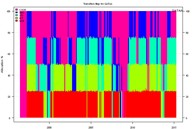
Let’s add another benchmark, for comparison we will use the Quantitative Approach To Tactical Asset Allocation Strategy(QATAA) by Mebane T. Faber
#*****************************************************************
#The [Quantitative Approach To Tactical Asset Allocation Strategy(QATAA) by Mebane T. Faber](http://mebfaber.com/timing-model/)
#[SSRN paper](http://papers.ssrn.com/sol3/papers.cfm?abstract_id=962461)
#******************************************************************
# compute 10 month moving average
sma = bt.apply.matrix(prices, SMA, 200)

# go to cash if prices falls below 10 month moving average
go2cash = prices < sma
  go2cash = ifna(go2cash, T)

# equal weight target allocation
target.allocation = ntop(prices,n)

# If asset is above it's 10 month moving average it gets allocation
weight = iif(go2cash, 0, target.allocation)

# otherwise, it's weight is allocated to cash
weight$CASH = 1 - rowSums(weight)

data$weight[] = NA
  data$weight[period.ends,] = weight[period.ends,]
models$QATAA = bt.run.share(data, clean.signal=F, commission = commission, trade.summary=T, silent=T)


#*****************************************************************
# Report
#*****************************************************************
#strategy.performance.snapshoot(models, T)
plotbt(models, plotX = T, log = 'y', LeftMargin = 3, main = NULL)
	mtext('Cumulative Performance', side = 2, line = 1)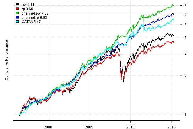
print(plotbt.strategy.sidebyside(models, make.plot=F, return.table=T))| ew | rp | channel.ew | channel.rp | QATAA | |
|---|---|---|---|---|---|
| Period | Jun1996 - Apr2015 | Jun1996 - Apr2015 | Jun1996 - Apr2015 | Jun1996 - Apr2015 | Jun1996 - Apr2015 |
| Cagr | 7.81 | 7.14 | 10.93 | 10.03 | 9.46 |
| Sharpe | 0.64 | 0.8 | 1.36 | 1.53 | 1.23 |
| DVR | 0.58 | 0.74 | 1.29 | 1.46 | 1.19 |
| Volatility | 13.16 | 9.2 | 7.87 | 6.38 | 7.64 |
| MaxDD | -48.78 | -40.52 | -12.81 | -7.95 | -13.71 |
| AvgDD | -1.52 | -1.21 | -1.16 | -1.01 | -1.06 |
| VaR | -1.07 | -0.76 | -0.74 | -0.61 | -0.7 |
| CVaR | -2.01 | -1.34 | -1.15 | -0.92 | -1.14 |
| Exposure | 99.98 | 99.51 | 99.98 | 99.98 | 99.98 |
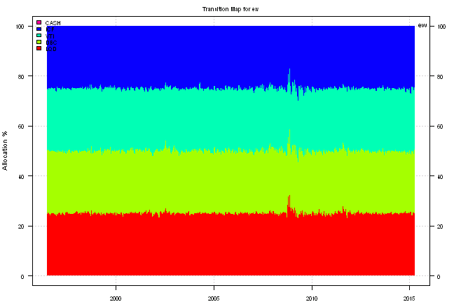
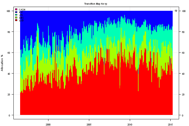
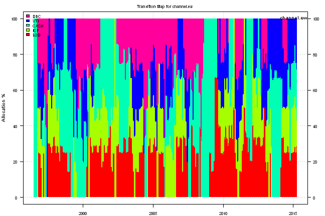
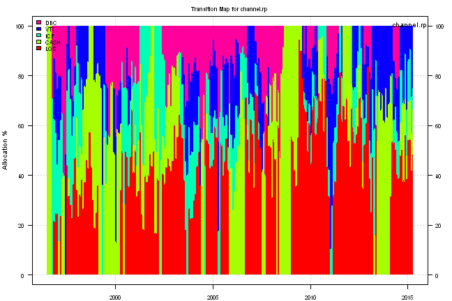
for(m in names(models)) {
  print('#', m, 'strategy:')
  plotbt.transition.map(models[[m]]$weight, name=m)
    legend('topright', legend = m, bty = 'n')

  print(plotbt.monthly.table(models[[m]]$equity, make.plot = F))

  print(to.percent(last(models[[m]]$weight)))
}
ew strategy:
| Jan | Feb | Mar | Apr | May | Jun | Jul | Aug | Sep | Oct | Nov | Dec | Year | MaxDD | |
|---|---|---|---|---|---|---|---|---|---|---|---|---|---|---|
| 1996 | -1.6 | 2.8 | 3.0 | 1.6 | 5.0 | 2.5 | 13.9 | -3.3 | ||||||
| 1997 | 1.4 | -0.4 | -1.0 | 1.1 | 3.4 | 1.8 | 4.8 | -1.6 | 4.9 | -0.7 | 0.2 | 0.3 | 14.7 | -4.9 |
| 1998 | -0.1 | 0.1 | 2.0 | -1.0 | -1.4 | 0.5 | -3.7 | -7.4 | 5.9 | -0.1 | 0.2 | 0.9 | -4.6 | -13.6 |
| 1999 | 0.4 | -3.3 | 4.3 | 4.2 | -1.5 | 2.3 | -1.5 | 0.8 | -0.3 | 0.2 | 1.2 | 3.2 | 10.2 | -4.8 |
| 2000 | 0.5 | 1.2 | 2.8 | -0.2 | 1.2 | 3.4 | 1.0 | 3.5 | -0.6 | -1.7 | -0.3 | 2.4 | 14.0 | -4.6 |
| 2001 | 1.8 | -2.8 | -2.8 | 3.3 | -0.1 | 0.1 | -0.2 | 0.1 | -5.5 | -0.5 | 3.0 | -0.2 | -3.9 | -11.3 |
| 2002 | -0.3 | 1.2 | 4.3 | -0.4 | 0.4 | -0.7 | -3.2 | 2.2 | -2.5 | 0.4 | 3.1 | 1.3 | 5.9 | -10.0 |
| 2003 | 0.4 | 2.0 | -1.3 | 3.2 | 4.8 | 0.8 | 1.0 | 2.3 | 1.4 | 2.2 | 1.7 | 4.1 | 24.9 | -3.4 |
| 2004 | 2.7 | 3.1 | 1.9 | -5.4 | 3.2 | -0.1 | 0.8 | 2.8 | 1.9 | 2.6 | 1.9 | 1.5 | 17.7 | -7.3 |
| 2005 | -2.1 | 2.8 | -0.2 | 0.0 | 1.6 | 2.3 | 4.0 | 0.5 | 0.1 | -2.7 | 2.4 | 1.8 | 10.8 | -4.4 |
| 2006 | 3.8 | -0.6 | 2.1 | 0.9 | -1.7 | 1.1 | 1.9 | 1.1 | 0.2 | 3.0 | 4.0 | -1.1 | 15.8 | -5.3 |
| 2007 | 2.3 | 0.6 | -0.6 | 1.7 | 0.1 | -3.2 | -2.5 | 2.1 | 4.7 | 3.0 | -3.5 | -0.1 | 4.3 | -7.8 |
| 2008 | -0.4 | 1.0 | 1.3 | 4.6 | 1.5 | -2.5 | -1.9 | -0.7 | -8.0 | -19.3 | -10.2 | 6.8 | -26.9 | -44.7 |
| 2009 | -8.2 | -11.3 | 4.0 | 11.5 | 6.9 | -0.9 | 6.1 | 3.9 | 3.3 | -0.3 | 4.9 | 1.8 | 21.1 | -24.9 |
| 2010 | -4.1 | 3.4 | 4.3 | 3.7 | -6.1 | -2.5 | 6.3 | -1.5 | 5.6 | 3.1 | -0.9 | 5.2 | 16.8 | -10.9 |
| 2011 | 2.4 | 3.3 | 0.2 | 3.9 | -0.8 | -2.6 | 1.6 | -2.9 | -8.4 | 9.1 | -2.0 | 1.5 | 4.4 | -14.8 |
| 2012 | 4.2 | 2.4 | 1.2 | 0.4 | -5.3 | 3.0 | 3.1 | 2.0 | 0.2 | -1.4 | 0.3 | 0.8 | 11.1 | -7.5 |
| 2013 | 2.3 | -0.6 | 1.7 | 1.7 | -2.2 | -2.3 | 2.5 | -2.0 | 1.0 | 2.4 | -1.0 | 0.9 | 4.3 | -7.9 |
| 2014 | 0.0 | 4.0 | 0.3 | 1.6 | 1.1 | 1.3 | -1.7 | 1.9 | -4.3 | 2.7 | -0.7 | -2.0 | 4.1 | -5.6 |
| 2015 | 0.6 | 1.1 | -1.3 | 0.5 | 0.9 | -3.4 | ||||||||
| Avg | 0.4 | 0.4 | 1.2 | 1.9 | 0.3 | 0.1 | 0.9 | 0.5 | 0.2 | 0.2 | 0.5 | 1.7 | 8.0 | -10.0 |
| LQD | DBC | VTI | ICF | CASH | |
|---|---|---|---|---|---|
| 2015-04-10 | 24.99% | 25.25% | 25.29% | 24.46% | 0.00% |
rp strategy:
| Jan | Feb | Mar | Apr | May | Jun | Jul | Aug | Sep | Oct | Nov | Dec | Year | MaxDD | |
|---|---|---|---|---|---|---|---|---|---|---|---|---|---|---|
| 1996 | -0.1 | 3.0 | 2.9 | 1.9 | 4.9 | 3.0 | 16.6 | -0.8 | ||||||
| 1997 | 1.1 | -0.4 | -0.7 | 1.0 | 2.9 | 2.2 | 4.7 | -1.5 | 5.3 | -0.7 | -0.4 | 0.2 | 14.3 | -4.7 |
| 1998 | -0.1 | -0.7 | 2.1 | -0.9 | -1.1 | 0.6 | -3.2 | -5.0 | 4.9 | -1.5 | -1.2 | 0.5 | -5.8 | -10.3 |
| 1999 | 0.2 | -3.1 | 3.1 | 3.9 | -1.6 | 1.6 | -1.6 | 0.4 | -0.3 | -0.5 | 0.3 | 2.3 | 4.4 | -4.8 |
| 2000 | 0.4 | 1.0 | 2.6 | 0.9 | 1.2 | 3.1 | 1.1 | 2.2 | -0.3 | -1.2 | 1.1 | 3.4 | 16.5 | -3.5 |
| 2001 | 1.8 | -1.7 | -1.9 | 1.6 | -0.2 | 1.2 | 0.3 | 1.2 | -4.5 | 0.5 | 2.2 | 0.2 | 0.5 | -7.9 |
| 2002 | -0.2 | 1.4 | 2.8 | 0.2 | 0.6 | 0.1 | -2.5 | 3.1 | -0.3 | -1.0 | 2.0 | 2.4 | 8.9 | -7.5 |
| 2003 | -0.5 | 2.3 | -0.4 | 2.6 | 4.5 | 0.5 | -0.2 | 2.3 | 1.8 | 1.4 | 1.5 | 3.6 | 21.1 | -2.6 |
| 2004 | 2.7 | 2.3 | 1.4 | -5.5 | 1.9 | 0.0 | 0.5 | 2.4 | 1.4 | 2.3 | 1.3 | 1.5 | 12.7 | -7.3 |
| 2005 | -1.6 | 1.5 | -0.7 | -0.2 | 1.5 | 1.8 | 3.1 | 0.7 | -0.7 | -2.2 | 1.5 | 1.6 | 6.3 | -3.7 |
| 2006 | 2.6 | -0.2 | 0.3 | 0.6 | -1.3 | 0.4 | 1.8 | 1.7 | 0.8 | 2.4 | 3.1 | -0.7 | 11.9 | -3.3 |
| 2007 | 1.4 | 0.5 | -0.6 | 1.3 | -0.1 | -1.5 | -1.7 | 1.8 | 4.0 | 2.7 | -2.1 | 0.1 | 5.8 | -4.8 |
| 2008 | 0.4 | 1.1 | 0.2 | 3.2 | 0.6 | -3.1 | -0.9 | -0.6 | -9.6 | -19.1 | -6.3 | 9.8 | -24.1 | -40.0 |
| 2009 | -4.6 | -7.9 | 2.6 | 5.6 | 5.1 | 0.8 | 5.5 | 2.5 | 2.4 | -0.3 | 3.8 | -0.3 | 15.2 | -17.2 |
| 2010 | -2.5 | 2.1 | 2.9 | 2.9 | -4.5 | 0.3 | 4.1 | 0.7 | 4.2 | 2.3 | -1.1 | 3.5 | 15.2 | -6.2 |
| 2011 | 2.1 | 2.7 | 0.0 | 3.3 | 0.1 | -1.6 | 1.8 | -1.9 | -5.9 | 5.6 | -2.5 | 2.2 | 5.5 | -9.3 |
| 2012 | 3.5 | 2.3 | 0.2 | 0.5 | -3.5 | 2.2 | 3.2 | 0.9 | 0.4 | -0.6 | -0.1 | 0.3 | 9.4 | -4.8 |
| 2013 | 1.3 | -0.1 | 0.9 | 2.1 | -2.8 | -2.5 | 2.5 | -1.2 | 0.7 | 2.4 | -0.6 | 0.9 | 3.5 | -7.2 |
| 2014 | 0.0 | 3.2 | 0.2 | 1.4 | 1.1 | 1.0 | -1.6 | 1.7 | -3.4 | 1.7 | 0.0 | -0.7 | 4.6 | -4.4 |
| 2015 | 1.9 | 0.0 | -0.9 | 0.5 | 1.5 | -3.1 | ||||||||
| Avg | 0.5 | 0.3 | 0.7 | 1.3 | 0.2 | 0.4 | 0.9 | 0.7 | 0.2 | -0.2 | 0.4 | 1.8 | 7.2 | -7.7 |
| LQD | DBC | VTI | ICF | CASH | |
|---|---|---|---|---|---|
| 2015-04-10 | 44.25% | 17.15% | 23.62% | 14.98% | 0.00% |
channel.ew strategy:
| Jan | Feb | Mar | Apr | May | Jun | Jul | Aug | Sep | Oct | Nov | Dec | Year | MaxDD | |
|---|---|---|---|---|---|---|---|---|---|---|---|---|---|---|
| 1996 | 0.3 | 0.1 | 1.1 | 0.9 | 5.0 | 2.5 | 10.2 | -1.2 | ||||||
| 1997 | 1.9 | -0.6 | -1.0 | -0.1 | 1.9 | -0.1 | 5.2 | -2.2 | 5.2 | -0.7 | -0.3 | 0.8 | 10.2 | -5.0 |
| 1998 | 0.4 | 1.3 | 1.9 | -0.4 | -0.5 | 1.6 | -0.7 | -2.6 | 2.4 | -0.3 | 0.1 | 2.1 | 5.4 | -4.4 |
| 1999 | 1.4 | -2.5 | 1.8 | 1.9 | -0.7 | 1.7 | -0.9 | 1.6 | 2.7 | -1.2 | 1.3 | 3.4 | 10.6 | -4.6 |
| 2000 | 0.3 | 2.0 | 2.2 | -2.4 | 1.7 | 2.5 | 2.0 | 2.6 | -0.6 | -1.7 | 2.6 | 1.8 | 13.7 | -6.0 |
| 2001 | 1.2 | -0.2 | -1.2 | -0.2 | 0.7 | 2.6 | 1.2 | 2.1 | -0.1 | 1.4 | -1.4 | -0.8 | 5.2 | -4.4 |
| 2002 | 0.1 | 1.0 | -0.3 | 0.4 | 1.3 | 1.3 | -0.6 | 2.3 | 1.7 | -0.2 | 0.1 | 2.9 | 10.2 | -6.2 |
| 2003 | 2.5 | 2.0 | -1.9 | 1.1 | 4.4 | 0.8 | 1.0 | 2.4 | 0.4 | 2.7 | 1.8 | 4.4 | 23.6 | -3.7 |
| 2004 | 2.7 | 3.1 | 1.9 | -5.9 | 2.3 | -3.4 | 2.2 | 4.0 | 1.7 | 2.8 | 1.9 | 1.5 | 15.2 | -7.5 |
| 2005 | -2.7 | 2.1 | 0.0 | -1.9 | 0.9 | 3.3 | 4.0 | 0.5 | 0.1 | -3.1 | -0.2 | 1.0 | 3.8 | -5.1 |
| 2006 | 4.5 | -0.8 | 3.0 | 0.2 | -1.6 | 0.8 | 2.4 | 1.0 | -0.4 | 3.2 | 2.8 | -0.7 | 15.0 | -5.3 |
| 2007 | 3.9 | -0.8 | -1.1 | 1.4 | 0.3 | -0.6 | -0.3 | 0.1 | 3.5 | 3.8 | -1.0 | 1.6 | 11.2 | -5.9 |
| 2008 | 2.2 | 3.0 | -0.4 | 1.9 | 1.8 | 6.9 | -3.0 | -0.6 | 0.5 | 1.1 | 1.1 | 0.5 | 15.7 | -5.4 |
| 2009 | -0.8 | -1.4 | 0.5 | 0.2 | 0.5 | 1.9 | 3.1 | 2.0 | 2.9 | -2.3 | 4.9 | 1.8 | 13.8 | -4.7 |
| 2010 | -4.1 | 3.3 | 3.6 | 3.7 | -5.5 | 0.4 | 2.5 | 1.0 | 1.5 | 1.9 | -1.0 | 6.3 | 13.7 | -9.1 |
| 2011 | 3.1 | 4.1 | 0.4 | 4.1 | -0.8 | -2.4 | 2.1 | -3.8 | 0.0 | 0.6 | -1.0 | 0.7 | 7.0 | -12.8 |
| 2012 | 0.5 | 0.1 | 2.2 | 1.0 | -2.9 | 1.8 | 1.9 | 0.3 | 0.3 | -1.5 | 0.2 | -0.2 | 3.7 | -5.3 |
| 2013 | 2.9 | -0.8 | 2.5 | 3.5 | -1.9 | -1.0 | 2.0 | -1.1 | 1.3 | 1.3 | 0.9 | 0.8 | 10.7 | -6.4 |
| 2014 | -1.0 | 1.8 | 0.2 | 1.3 | 1.1 | 1.3 | -1.7 | 2.6 | -2.5 | 1.4 | 1.5 | 0.3 | 6.4 | -4.0 |
| 2015 | 2.2 | -0.9 | 0.3 | 0.2 | 1.8 | -3.6 | ||||||||
| Avg | 1.1 | 0.8 | 0.8 | 0.5 | 0.2 | 1.1 | 1.2 | 0.6 | 1.1 | 0.5 | 1.0 | 1.6 | 10.4 | -5.5 |
| LQD | DBC | VTI | ICF | CASH | |
|---|---|---|---|---|---|
| 2015-04-10 | 28.57% | 0.00% | 28.91% | 13.98% | 28.54% |
channel.rp strategy:
| Jan | Feb | Mar | Apr | May | Jun | Jul | Aug | Sep | Oct | Nov | Dec | Year | MaxDD | |
|---|---|---|---|---|---|---|---|---|---|---|---|---|---|---|
| 1996 | 0.3 | 0.1 | 1.1 | 1.6 | 4.9 | 3.0 | 11.4 | -1.0 | ||||||
| 1997 | 1.7 | -0.5 | -0.7 | 0.0 | 1.9 | -0.5 | 5.0 | -1.9 | 5.7 | -0.7 | -0.6 | 0.8 | 10.3 | -4.6 |
| 1998 | 0.4 | 0.3 | 2.0 | -0.7 | -0.2 | 1.6 | -0.7 | -1.0 | 2.7 | -0.8 | 0.3 | 1.7 | 5.7 | -3.6 |
| 1999 | 1.2 | -2.6 | 1.3 | 1.2 | -0.6 | 0.9 | -0.9 | 1.2 | 2.5 | -0.9 | 0.7 | 2.5 | 6.5 | -4.5 |
| 2000 | 0.4 | 1.7 | 1.6 | -1.7 | 0.7 | 2.5 | 1.8 | 1.5 | -0.3 | -1.2 | 2.1 | 2.5 | 12.2 | -3.2 |
| 2001 | 1.6 | -0.4 | -0.9 | -0.5 | 0.7 | 3.5 | 1.3 | 2.3 | -0.2 | 2.1 | -1.5 | -0.9 | 7.1 | -4.8 |
| 2002 | 0.1 | 1.3 | 0.0 | 0.4 | 1.4 | 1.2 | -1.4 | 3.1 | 1.9 | -0.3 | 0.4 | 3.2 | 11.7 | -7.9 |
| 2003 | 0.8 | 2.1 | -0.9 | 1.7 | 4.3 | 0.5 | -0.2 | 2.4 | 0.7 | 2.0 | 1.7 | 4.0 | 20.5 | -3.1 |
| 2004 | 2.7 | 2.3 | 1.4 | -5.8 | 1.8 | -2.4 | 1.3 | 3.4 | 1.2 | 2.4 | 1.3 | 1.5 | 11.4 | -7.0 |
| 2005 | -1.9 | 0.8 | -0.6 | -2.5 | 1.5 | 2.5 | 3.1 | 0.7 | -0.7 | -2.4 | 0.1 | 0.9 | 1.2 | -5.5 |
| 2006 | 3.6 | -0.6 | 2.0 | 0.4 | -1.2 | 0.4 | 1.5 | 0.9 | 0.3 | 2.4 | 2.6 | -0.5 | 12.6 | -2.6 |
| 2007 | 2.0 | -0.4 | -0.8 | 1.1 | 0.1 | -0.9 | 0.0 | 0.1 | 5.8 | 3.0 | -0.6 | 1.1 | 10.7 | -3.7 |
| 2008 | 2.4 | 2.1 | -0.5 | 1.7 | 0.3 | 5.3 | -1.5 | -0.2 | 0.5 | 1.1 | 1.1 | 0.5 | 13.3 | -3.6 |
| 2009 | -1.2 | -2.9 | 0.5 | 0.8 | 1.3 | 2.7 | 4.1 | 1.8 | 2.2 | -1.4 | 3.8 | -0.3 | 11.7 | -5.8 |
| 2010 | -2.5 | 1.8 | 2.0 | 2.7 | -3.9 | 2.1 | 2.0 | 2.2 | 1.0 | 0.6 | -1.1 | 4.8 | 12.0 | -5.5 |
| 2011 | 2.6 | 4.0 | 0.1 | 3.6 | 0.0 | -1.5 | 2.3 | -2.2 | 0.2 | 1.5 | -2.2 | 1.9 | 10.5 | -7.3 |
| 2012 | 0.9 | 0.7 | 0.7 | 1.0 | -1.4 | 1.3 | 2.8 | 0.1 | 0.5 | -0.5 | -0.2 | -0.3 | 5.6 | -3.7 |
| 2013 | 1.8 | -0.3 | 1.6 | 3.6 | -2.6 | -0.8 | 1.6 | -1.1 | 1.2 | 1.6 | 0.7 | 0.9 | 8.3 | -5.2 |
| 2014 | -0.9 | 1.3 | 0.1 | 1.2 | 1.1 | 1.0 | -1.6 | 2.3 | -2.1 | 1.4 | 1.2 | 0.2 | 5.2 | -3.0 |
| 2015 | 2.9 | -1.3 | 0.0 | 0.4 | 1.9 | -3.1 | ||||||||
| Avg | 1.0 | 0.5 | 0.5 | 0.4 | 0.3 | 1.1 | 1.1 | 0.8 | 1.3 | 0.6 | 0.8 | 1.4 | 9.5 | -4.4 |
| LQD | DBC | VTI | ICF | CASH | |
|---|---|---|---|---|---|
| 2015-04-10 | 47.94% | 0.00% | 25.59% | 8.11% | 18.37% |
QATAA strategy:
| Jan | Feb | Mar | Apr | May | Jun | Jul | Aug | Sep | Oct | Nov | Dec | Year | MaxDD | |
|---|---|---|---|---|---|---|---|---|---|---|---|---|---|---|
| 1996 | 0.3 | 0.1 | 1.2 | 1.5 | 1.1 | -0.5 | 3.8 | -1.0 | ||||||
| 1997 | 0.4 | 0.0 | -0.6 | 0.9 | 3.4 | 1.8 | 4.8 | -1.6 | 4.9 | -0.7 | 0.1 | 1.6 | 15.8 | -4.1 |
| 1998 | 0.4 | 1.3 | 2.0 | -0.4 | -0.3 | 1.5 | -0.6 | -2.6 | 2.4 | -0.3 | 1.8 | 1.9 | 7.2 | -4.2 |
| 1999 | 1.4 | -2.5 | 1.3 | 1.8 | -1.2 | 2.6 | -1.2 | 0.9 | -0.3 | -1.0 | 1.7 | 2.5 | 6.0 | -3.2 |
| 2000 | 0.0 | 1.8 | 2.2 | -0.2 | 1.2 | 3.0 | 1.0 | 3.5 | -0.6 | -1.7 | 2.5 | 2.4 | 16.0 | -4.6 |
| 2001 | 1.2 | -0.2 | -1.0 | 0.1 | -0.2 | 1.8 | 1.2 | 2.1 | -0.1 | 0.8 | -1.3 | -0.2 | 4.1 | -3.7 |
| 2002 | 0.3 | 1.0 | -0.3 | -0.4 | 0.9 | 1.4 | -0.5 | 2.2 | 0.2 | -0.2 | 0.1 | 3.1 | 7.8 | -3.3 |
| 2003 | 1.8 | 2.0 | -1.9 | 1.0 | 4.8 | 0.8 | 1.0 | 2.3 | 1.4 | 2.2 | 1.7 | 4.1 | 23.3 | -3.7 |
| 2004 | 2.7 | 3.1 | 1.9 | -5.5 | 1.3 | -0.1 | 0.4 | 2.7 | 1.4 | 2.6 | 1.9 | 1.5 | 14.5 | -6.5 |
| 2005 | -2.1 | 2.8 | -0.2 | 0.0 | 1.6 | 2.3 | 4.0 | 0.5 | 0.1 | -2.8 | 2.3 | 1.6 | 10.6 | -4.4 |
| 2006 | 3.8 | -0.7 | 2.1 | 1.0 | -1.6 | 1.2 | 1.7 | 1.1 | 0.2 | 2.9 | 2.5 | -1.1 | 13.7 | -5.3 |
| 2007 | 2.3 | -0.5 | -0.6 | 1.7 | 0.1 | -3.2 | 0.0 | 0.4 | 3.6 | 2.9 | -0.6 | 1.2 | 7.3 | -5.4 |
| 2008 | 2.2 | 3.0 | -0.4 | 1.4 | 0.9 | -0.2 | -2.1 | -1.3 | -2.7 | 1.1 | 1.1 | 0.5 | 3.3 | -9.5 |
| 2009 | -0.8 | -1.4 | 0.5 | 0.6 | 0.6 | 0.7 | 3.5 | 3.9 | 3.3 | -0.3 | 4.9 | 1.8 | 18.3 | -5.1 |
| 2010 | -4.1 | 2.4 | 4.3 | 3.7 | -6.1 | -1.9 | 3.2 | 0.6 | 1.1 | 3.1 | -0.9 | 5.2 | 10.2 | -10.0 |
| 2011 | 2.4 | 3.3 | 0.2 | 3.9 | -0.8 | -2.6 | 1.6 | -2.9 | -6.5 | 0.6 | -1.8 | 0.9 | -2.2 | -13.7 |
| 2012 | 3.3 | 1.0 | 1.2 | 0.4 | -5.4 | 2.5 | 1.7 | 0.5 | 0.2 | -1.5 | -0.2 | -0.1 | 3.5 | -7.2 |
| 2013 | 2.3 | -0.6 | 1.6 | 2.7 | -1.9 | -0.8 | 1.5 | -2.5 | 1.1 | 1.1 | 0.7 | 0.6 | 5.8 | -6.0 |
| 2014 | -0.3 | 1.5 | 0.3 | 1.6 | 1.1 | 1.3 | -1.7 | 2.3 | -2.5 | 3.7 | 1.5 | 0.3 | 9.3 | -2.7 |
| 2015 | 2.2 | -0.1 | 0.3 | -0.1 | 2.3 | -2.8 | ||||||||
| Avg | 1.0 | 0.9 | 0.7 | 0.8 | -0.1 | 0.7 | 1.0 | 0.6 | 0.4 | 0.7 | 1.0 | 1.4 | 9.0 | -5.3 |
| LQD | DBC | VTI | ICF | CASH | |
|---|---|---|---|---|---|
| 2015-04-10 | 25.07% | 0.00% | 25.37% | 24.53% | 25.04% |
# plotbt(models[3], xfun = function(x) { 100 * compute.drawdown(x$equity) })Finnally, let’s zoom in on the recent perfomance strating in 2010:
models.2010 = bt.trim(models, dates = '2010::')

plotbt(models.2010, plotX = T, log = 'y', LeftMargin = 3, main = NULL)
	mtext('Cumulative Performance', side = 2, line = 1)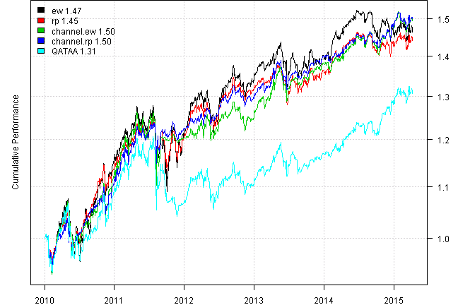
print(plotbt.strategy.sidebyside(models.2010, make.plot=F, return.table=T))| ew | rp | channel.ew | channel.rp | QATAA | |
|---|---|---|---|---|---|
| Period | Jan2010 - Apr2015 | Jan2010 - Apr2015 | Jan2010 - Apr2015 | Jan2010 - Apr2015 | Jan2010 - Apr2015 |
| Cagr | 7.58 | 7.24 | 7.96 | 8.02 | 5.24 |
| Sharpe | 0.71 | 0.98 | 0.9 | 1.24 | 0.63 |
| DVR | 0.65 | 0.91 | 0.85 | 1.19 | 0.47 |
| Volatility | 11.41 | 7.6 | 9.15 | 6.55 | 9.11 |
| MaxDD | -14.76 | -9.27 | -12.81 | -7.3 | -13.71 |
| AvgDD | -1.64 | -1.2 | -1.39 | -1.09 | -1.57 |
| VaR | -1.11 | -0.73 | -0.83 | -0.61 | -0.92 |
| CVaR | -1.74 | -1.12 | -1.42 | -0.99 | -1.45 |
| Exposure | 100 | 100 | 100 | 100 | 100 |
David, thank you for another interesting concept.
Just a quick update with new code for Channel function. I.e. fix for a lower channel outlined at Run Channel in Rcpp Update post.
#*****************************************************************
# Strategy:
#
# 1) Use 60,120,180, 252-day percentile channels
# - corresponding to 3,6,9 and 12 months in the momentum literature-
# (4 separate systems) with a .75 long entry and .25 exit threshold with
# long triggered above .75 and holding through until exiting below .25
# (just like in the previous post) - no shorts!!!
#
# 2) If the indicator shows that you should be in cash, hold SHY
#
# 3) Use 20-day historical volatility for risk parity position-sizing
# among active assets (no leverage is used). This is 1/volatility (asset A)
# divided by the sum of 1/volatility for all assets to determine the position size.
#******************************************************************

# load conditional qunatile function developed in the [Run Channel in Rcpp Update](/Run-Channel-Rcpp-Update) post
load.packages('Rcpp')
# you can download `channel1.cpp` file at [channel1.cpp](/public/doc/channel1.cpp)
sourceCpp('channel1.cpp')

allocation = 0 * ifna(prices, 0)
for(lookback.len in c(60,120,180, 252)) {
  channels = bt.apply.matrix.ex2(prices, run_quantile_weight, lookback.len, 0.25, 0.75)
  signal = iif(cross.up(prices, channels$high), 1, iif(cross.dn(prices, channels$low), -1, NA))
  allocation = allocation + ifna( bt.apply.matrix(signal, ifna.prev), 0)
}

# (A) Channel score
allocation = ifna(allocation / 4, 0)

# equal-weight
weight = abs(allocation) / rowSums(abs(allocation))
	weight[allocation < 0] = 0
weight$CASH = 1 - rowSums(weight, na.rm=T)

data$weight[] = NA
  data$weight[period.ends,] = weight[period.ends,]
models$channel.ew = bt.run.share(data, clean.signal=F, commission = commission, trade.summary=T, silent=T)


# risk-parity: (C)
weight = allocation * 1 / hist.vol
weight = abs(weight) / rowSums(abs(weight), na.rm=T)
	weight[allocation < 0] = 0
weight$CASH = 1 - rowSums(weight, na.rm=T)

data$weight[] = NA
  data$weight[period.ends,] = ifna(weight[period.ends,], 0)
models$channel.rp = bt.run.share(data, clean.signal=F, commission = commission, trade.summary=T, silent=T)

#*****************************************************************
# Report
#*****************************************************************
#strategy.performance.snapshoot(models, T)
plotbt(models, plotX = T, log = 'y', LeftMargin = 3, main = NULL)
	mtext('Cumulative Performance', side = 2, line = 1)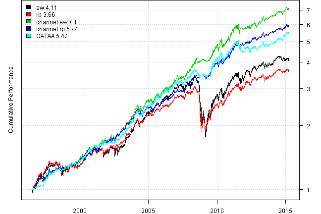
print(plotbt.strategy.sidebyside(models, make.plot=F, return.table=T))| ew | rp | channel.ew | channel.rp | QATAA | |
|---|---|---|---|---|---|
| Period | Jun1996 - Apr2015 | Jun1996 - Apr2015 | Jun1996 - Apr2015 | Jun1996 - Apr2015 | Jun1996 - Apr2015 |
| Cagr | 7.81 | 7.14 | 11.01 | 9.94 | 9.46 |
| Sharpe | 0.64 | 0.8 | 1.38 | 1.53 | 1.23 |
| DVR | 0.58 | 0.74 | 1.31 | 1.46 | 1.19 |
| Volatility | 13.16 | 9.2 | 7.81 | 6.36 | 7.64 |
| MaxDD | -48.78 | -40.52 | -12.79 | -8.33 | -13.71 |
| AvgDD | -1.52 | -1.21 | -1.15 | -1.01 | -1.06 |
| VaR | -1.07 | -0.76 | -0.75 | -0.6 | -0.7 |
| CVaR | -2.01 | -1.34 | -1.15 | -0.92 | -1.14 |
| Exposure | 99.98 | 99.51 | 99.98 | 99.98 | 99.98 |
models.2010 = bt.trim(models, dates = '2010::')

plotbt(models.2010, plotX = T, log = 'y', LeftMargin = 3, main = NULL)
	mtext('Cumulative Performance', side = 2, line = 1)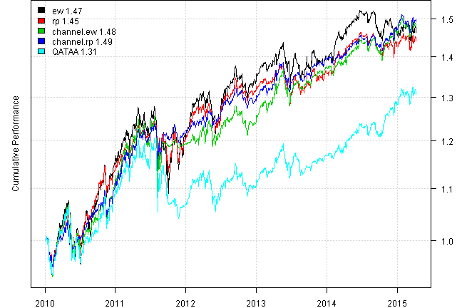
print(plotbt.strategy.sidebyside(models.2010, make.plot=F, return.table=T))| ew | rp | channel.ew | channel.rp | QATAA | |
|---|---|---|---|---|---|
| Period | Jan2010 - Apr2015 | Jan2010 - Apr2015 | Jan2010 - Apr2015 | Jan2010 - Apr2015 | Jan2010 - Apr2015 |
| Cagr | 7.58 | 7.24 | 7.77 | 7.93 | 5.24 |
| Sharpe | 0.71 | 0.98 | 0.89 | 1.23 | 0.63 |
| DVR | 0.65 | 0.91 | 0.84 | 1.18 | 0.47 |
| Volatility | 11.41 | 7.6 | 9.11 | 6.54 | 9.11 |
| MaxDD | -14.76 | -9.27 | -12.79 | -7.91 | -13.71 |
| AvgDD | -1.64 | -1.2 | -1.39 | -1.1 | -1.57 |
| VaR | -1.11 | -0.73 | -0.85 | -0.61 | -0.92 |
| CVaR | -1.74 | -1.12 | -1.42 | -0.99 | -1.45 |
| Exposure | 100 | 100 | 100 | 100 | 100 |
(this report was produced on: 2015-04-13)