Thinking in SIT, more examples
24 Feb 2015To install Systematic Investor Toolbox (SIT) please visit About page.
I previously presented a case study of Excel to SIT mapping in the Thinking in SIT post. I want to continue with another example based on following excellent tutorials:
- Backtesting A Basic ETF Rotation System in Excel Free Download
- Improving the Simple ETF Rotational Trading Model
The Backtesting A Basic ETF Rotation System in Excel Free Download was covered in the Thinking in SIT post.
Following is the code for your reference:
#*****************************************************************
# Load historical data
#*****************************************************************
library(SIT)
load.packages('quantmod')

# load saved Proxies Raw Data, data.proxy.raw
# please see http://systematicinvestor.github.io/Data-Proxy/ for more details
load('data/data.proxy.raw.Rdata')

tickers = '
EQ = SPY # S&P 500
GOLD = GLD + GOLD # Gold
GOV.10YR = IEF + VFITX # 10 Year Treasury
RE = IYR + VGSIX # US Real Estate
EM = EEM + VEIEX # Emerging Markets
CASH = SHY + TB3Y # CASH
'

data <- new.env()
getSymbols.extra(tickers, src = 'yahoo', from = '1970-01-01', env = data, raw.data = data.proxy.raw, set.symbolnames = T, auto.assign = T)
for(i in data$symbolnames) data[[i]] = adjustOHLC(data[[i]], use.Adjusted=T)
bt.prep(data, align='remove.na')

# Check data
plota.matplot(scale.one(data$prices),main='Asset Perfromance')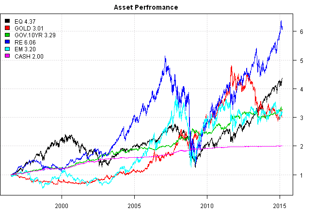
#*****************************************************************
# Code Strategies
#*****************************************************************
data$universe = data$prices > 0
  # do not allocate to CASH
  data$universe$CASH = NA

prices = data$prices * data$universe
  n = ncol(prices)
  nperiods = nrow(prices)

# find period ends, can be 'weeks', 'months', 'quarters', 'years'
frequency = 'months'
period.ends = endpoints(prices, frequency)
  period.ends = period.ends[period.ends > 0]

commission = list(cps = 0.01, fixed = 10.0, percentage = 0.0)

models = list()

#*****************************************************************
# Code Strategies, SPY - Buy & Hold
#*****************************************************************
data$weight[] = NA
	data$weight$EQ = 1
models$SP500 = bt.run.share(data, clean.signal=T, commission = commission, trade.summary=T, silent=T)

#*****************************************************************
# Code Strategies, Equal Weight, re-balanced monthly
#*****************************************************************
data$weight[] = NA
	data$weight[period.ends,] = ntop(prices, n)[period.ends,]
models$EW = bt.run.share(data, clean.signal=F, commission = commission, trade.summary=T, silent=T)

#*****************************************************************
# Code Strategies, Top 1 based on 5 month momentum, re-balanced monthly
#
# alternatively to compute real 5 month return based on month ends
# position.score = bt.apply.matrix(prices, function(x) x / mlag(x,5), periodicity='months')
#*****************************************************************
position.score = prices / mlag(prices, 5*21)

data$weight[] = NA
	data$weight[period.ends,] = ntop(position.score[period.ends,], 1)
models$TOP1 = bt.run.share(data, clean.signal=F, commission = commission, trade.summary=T, silent=T)

#*****************************************************************
# Create Report
#*****************************************************************
plotbt(models, plotX = T, log = 'y', LeftMargin = 3, main = NULL)
	mtext('Cumulative Performance', side = 2, line = 1)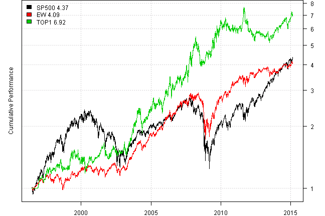
print(plotbt.strategy.sidebyside(models, make.plot=F, return.table=T, perfromance.fn=engineering.returns.kpi))| SP500 | EW | TOP1 | |
|---|---|---|---|
| Period | Jun1996 - Feb2015 | Jun1996 - Feb2015 | Jun1996 - Feb2015 |
| Cagr | 8.22 | 7.83 | 10.92 |
| Sharpe | 0.5 | 0.64 | 0.65 |
| DVR | 0.29 | 0.58 | 0.59 |
| R2 | 0.58 | 0.92 | 0.9 |
| Volatility | 20.27 | 13.44 | 18.79 |
| MaxDD | -55.19 | -40.79 | -32.76 |
| Exposure | 99.98 | 99.98 | 97.7 |
| Win.Percent | 100 | 58.85 | 58.72 |
| Avg.Trade | 336.9 | 0.15 | 1.04 |
| Profit.Factor | NaN | 1.49 | 1.73 |
| Num.Trades | 1 | 1113 | 218 |
print(last.trades(models$TOP1, make.plot=F, return.table=T))| models$TOP1 | weight | entry.date | exit.date | nhold | entry.price | exit.price | return |
|---|---|---|---|---|---|---|---|
| EQ | 100 | 2013-06-28 | 2013-07-31 | 33 | 155.74 | 163.78 | 5.16 |
| EQ | 100 | 2013-07-31 | 2013-08-30 | 30 | 163.78 | 158.87 | -3.00 |
| EQ | 100 | 2013-08-30 | 2013-09-30 | 31 | 158.87 | 163.90 | 3.17 |
| EQ | 100 | 2013-09-30 | 2013-10-31 | 31 | 163.90 | 171.49 | 4.63 |
| EQ | 100 | 2013-10-31 | 2013-11-29 | 29 | 171.49 | 176.57 | 2.96 |
| EQ | 100 | 2013-11-29 | 2013-12-31 | 32 | 176.57 | 181.15 | 2.59 |
| EQ | 100 | 2013-12-31 | 2014-01-31 | 31 | 181.15 | 174.77 | -3.52 |
| EQ | 100 | 2014-01-31 | 2014-02-28 | 28 | 174.77 | 182.72 | 4.55 |
| EQ | 100 | 2014-02-28 | 2014-03-31 | 31 | 182.72 | 184.24 | 0.83 |
| EQ | 100 | 2014-03-31 | 2014-04-30 | 30 | 184.24 | 185.52 | 0.69 |
| RE | 100 | 2014-04-30 | 2014-05-30 | 30 | 67.81 | 69.70 | 2.79 |
| RE | 100 | 2014-05-30 | 2014-06-30 | 31 | 69.70 | 70.41 | 1.02 |
| EM | 100 | 2014-06-30 | 2014-07-31 | 31 | 42.62 | 43.20 | 1.36 |
| EM | 100 | 2014-07-31 | 2014-08-29 | 29 | 43.20 | 44.42 | 2.82 |
| RE | 100 | 2014-08-29 | 2014-09-30 | 32 | 72.77 | 68.49 | -5.88 |
| EQ | 100 | 2014-09-30 | 2014-10-31 | 31 | 195.94 | 200.55 | 2.35 |
| RE | 100 | 2014-10-31 | 2014-11-28 | 28 | 74.21 | 76.23 | 2.72 |
| RE | 100 | 2014-11-28 | 2014-12-31 | 33 | 76.23 | 76.84 | 0.80 |
| RE | 100 | 2014-12-31 | 2015-01-30 | 30 | 76.84 | 81.23 | 5.71 |
| RE | 100 | 2015-01-30 | 2015-02-24 | 25 | 81.23 | 79.06 | -2.67 |
In the Improving the Simple ETF Rotational Trading Model post, Jeff Swanson, showcases a few simple rules you might use to improve performance and reduce draw downs.
Modification 1: Diversification and Trend Filter
#*****************************************************************
# Modification 1: Diversification and Trend Filter
#
# - Buying the top two performing ETFs
# - Buying only when an ETF is trading above its 5-month simple moving average
#*****************************************************************
# compute 5 month moving average
sma = bt.apply.matrix(prices, SMA, 5*21)
go2cash = prices < sma
  go2cash = ifna(go2cash, T)[period.ends,]

# rank assets by 5 month return
position.score = prices / mlag(prices, 5*21)

# select top 2 assets
weight = ntop(position.score[period.ends,], 2)

# if selected asset is below 5 month moving average, move allocation to CASH
weight = iif(go2cash, 0, weight)
weight$CASH = 1 - rowSums(weight, na.rm=T)

data$weight[] = NA
	data$weight[period.ends,] = weight
models$TOP2.CASH = bt.run.share(data, clean.signal=F, commission = commission, trade.summary=T, silent=T)
Modification 2: Adjusting the Ranking Score
#*****************************************************************
# Modification 2: Adjusting the Ranking Score
# same as Modification 1, plus
# ranking is based on average of 3-month and 20-day returns
#*****************************************************************
position.score = prices / mlag(prices, 3*21) + prices / mlag(prices, 21)

# select top 2 assets
weight = ntop(position.score[period.ends,], 2)

# if selected asset is below 5 month moving average, move allocation to CASH
weight = iif(go2cash, 0, weight)
weight$CASH = 1 - rowSums(weight, na.rm=T)

data$weight[] = NA
	data$weight[period.ends,] = weight
models$AVG.TOP2.CASH = bt.run.share(data, clean.signal=F, commission = commission, trade.summary=T, silent=T)
Let’s look at the performance:
#*****************************************************************
# Create Report
#*****************************************************************
plotbt(models, plotX = T, log = 'y', LeftMargin = 3, main = NULL)
	mtext('Cumulative Performance', side = 2, line = 1)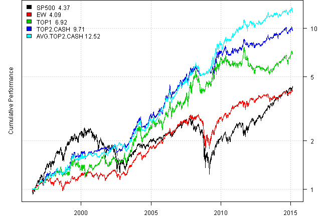
print(plotbt.strategy.sidebyside(models, make.plot=F, return.table=T, perfromance.fn=engineering.returns.kpi))| SP500 | EW | TOP1 | TOP2.CASH | AVG.TOP2.CASH | |
|---|---|---|---|---|---|
| Period | Jun1996 - Feb2015 | Jun1996 - Feb2015 | Jun1996 - Feb2015 | Jun1996 - Feb2015 | Jun1996 - Feb2015 |
| Cagr | 8.22 | 7.83 | 10.92 | 12.94 | 14.49 |
| Sharpe | 0.5 | 0.64 | 0.65 | 0.99 | 1.05 |
| DVR | 0.29 | 0.58 | 0.59 | 0.92 | 0.93 |
| R2 | 0.58 | 0.92 | 0.9 | 0.93 | 0.88 |
| Volatility | 20.27 | 13.44 | 18.79 | 13.43 | 13.97 |
| MaxDD | -55.19 | -40.79 | -32.76 | -17.61 | -17.61 |
| Exposure | 99.98 | 99.98 | 97.7 | 99.98 | 99.98 |
| Win.Percent | 100 | 58.85 | 58.72 | 62.61 | 64.07 |
| Avg.Trade | 336.9 | 0.15 | 1.04 | 0.58 | 0.64 |
| Profit.Factor | NaN | 1.49 | 1.73 | 2.01 | 2.12 |
| Num.Trades | 1 | 1113 | 218 | 436 | 437 |
print(plotbt.monthly.table(models$AVG.TOP2.CASH$equity, make.plot = F))| Jan | Feb | Mar | Apr | May | Jun | Jul | Aug | Sep | Oct | Nov | Dec | Year | MaxDD | |
|---|---|---|---|---|---|---|---|---|---|---|---|---|---|---|
| 1996 | 0.3 | 0.1 | 1.2 | 1.5 | 1.0 | 4.8 | 9.2 | -1.6 | ||||||
| 1997 | 2.7 | 0.2 | 0.0 | -3.8 | 3.5 | 4.0 | 4.7 | -3.1 | 5.3 | -2.7 | 1.0 | 2.2 | 14.2 | -8.7 |
| 1998 | -0.2 | 3.2 | 4.3 | 0.1 | -7.4 | 2.6 | -0.6 | -2.7 | 3.4 | -0.8 | 5.9 | 1.6 | 9.1 | -9.6 |
| 1999 | 0.3 | -3.2 | 7.9 | 9.5 | -1.1 | 3.0 | -3.3 | -0.5 | 0.7 | 0.0 | -0.5 | 6.8 | 20.2 | -7.6 |
| 2000 | -4.9 | 0.9 | -0.1 | 1.6 | 0.5 | 3.2 | 1.2 | 0.0 | -1.2 | -2.5 | 1.8 | 1.6 | 1.8 | -8.2 |
| 2001 | 0.7 | -5.1 | 0.2 | 1.1 | 1.4 | 3.1 | -0.1 | 1.8 | -1.1 | -1.3 | -1.9 | 4.5 | 2.8 | -6.8 |
| 2002 | 0.5 | 2.3 | 2.9 | 0.3 | 3.9 | -0.5 | -1.2 | 1.4 | 3.6 | -1.7 | -1.4 | -4.3 | 5.6 | -7.7 |
| 2003 | 3.0 | -4.7 | -2.1 | 1.7 | 7.3 | 2.6 | 3.7 | 4.4 | 1.3 | 4.3 | 2.5 | 6.1 | 33.8 | -9.9 |
| 2004 | 3.5 | 2.8 | 2.9 | -11.7 | 0.0 | -0.1 | -1.5 | 5.5 | 0.8 | 4.0 | 7.0 | 0.9 | 13.6 | -15.4 |
| 2005 | -4.6 | 5.9 | -5.0 | 0.5 | 2.8 | 2.4 | 7.1 | -1.5 | 8.1 | -3.5 | 3.0 | 5.6 | 21.5 | -8.1 |
| 2006 | 12.0 | -2.5 | 2.8 | 4.3 | -6.3 | -2.3 | 3.4 | 2.4 | 1.7 | 4.8 | 5.3 | 1.8 | 29.8 | -17.6 |
| 2007 | 4.9 | -3.5 | -0.7 | 2.8 | 4.2 | 1.1 | -1.2 | 1.6 | 5.8 | 9.4 | -4.7 | 3.3 | 24.5 | -11.3 |
| 2008 | 7.1 | 3.2 | -2.3 | -3.4 | 2.0 | -10.5 | -0.5 | 1.0 | 0.2 | 0.1 | 1.1 | 2.8 | -0.4 | -16.7 |
| 2009 | 0.8 | 0.3 | 0.3 | 7.6 | 9.1 | -2.4 | 10.8 | 5.9 | 4.8 | -4.3 | 9.9 | -2.0 | 47.3 | -11.9 |
| 2010 | -6.6 | 2.8 | 7.9 | 3.9 | -1.4 | 2.7 | -2.1 | 0.0 | 2.3 | 3.4 | -0.5 | 4.5 | 17.4 | -9.8 |
| 2011 | 2.9 | 4.0 | -0.6 | 3.7 | -0.4 | -1.8 | 1.6 | 8.4 | -4.5 | -0.7 | -2.1 | 1.5 | 12.0 | -15.4 |
| 2012 | 5.6 | -1.9 | 0.0 | 0.9 | -5.1 | 2.5 | 1.8 | 0.1 | 0.6 | -1.7 | 0.5 | 2.1 | 5.2 | -8.8 |
| 2013 | 1.8 | 1.3 | 3.3 | 3.8 | -2.1 | -0.7 | 2.6 | -1.6 | -0.9 | 4.4 | 1.3 | 1.1 | 15.0 | -7.4 |
| 2014 | -6.1 | 2.5 | -1.5 | 1.9 | 2.9 | 1.7 | -1.2 | 3.1 | -4.6 | 1.9 | 2.7 | 0.3 | 2.9 | -6.8 |
| 2015 | 1.3 | -4.7 | -3.4 | -7.2 | ||||||||||
| Avg | 1.3 | 0.2 | 1.1 | 1.4 | 0.8 | 0.6 | 1.3 | 1.4 | 1.5 | 0.8 | 1.7 | 2.4 | 14.1 | -9.8 |
Finnally, let’s zoom in on the last 2 years:
models1 = bt.trim(models, dates = '2013::')

plotbt(models1, plotX = T, log = 'y', LeftMargin = 3, main = NULL)
	mtext('Cumulative Performance', side = 2, line = 1)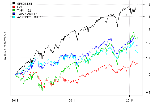
print(plotbt.strategy.sidebyside(models1, make.plot=F, return.table=T, perfromance.fn=engineering.returns.kpi))| SP500 | EW | TOP1 | TOP2.CASH | AVG.TOP2.CASH | |
|---|---|---|---|---|---|
| Period | Jan2013 - Feb2015 | Jan2013 - Feb2015 | Jan2013 - Feb2015 | Jan2013 - Feb2015 | Jan2013 - Feb2015 |
| Cagr | 21.12 | 2.91 | 9.54 | 8 | 5.59 |
| Sharpe | 1.84 | 0.44 | 0.89 | 0.9 | 0.65 |
| DVR | 1.79 | 0.19 | 0.75 | 0.78 | 0.49 |
| R2 | 0.97 | 0.42 | 0.85 | 0.86 | 0.74 |
| Volatility | 11.4 | 8.75 | 12.1 | 10.26 | 10.45 |
| MaxDD | -7.27 | -10.67 | -12.21 | -9.27 | -7.35 |
| Exposure | 100 | 100 | 100 | 100 | 100 |
| Win.Percent | 100 | 58.85 | 58.72 | 62.61 | 64.07 |
| Avg.Trade | 336.9 | 0.15 | 1.04 | 0.58 | 0.64 |
| Profit.Factor | NaN | 1.49 | 1.73 | 2.01 | 2.12 |
| Num.Trades | 1 | 1113 | 218 | 436 | 437 |
Please experiment and have fun.
Revolution Analytics put the An R tutorial for Microsoft Excel users post that highlights following useful resources:
(this report was produced on: 2015-02-25)