Exponentially Weighted Volatility using RCPP
10 Apr 2016To install Systematic Investor Toolbox (SIT) please visit About page.
The Exponentially Weighted Volatility is a measure of volatility that put more weight on the recent observations. We will use following formula to compute the Exponentially Weighted Volatility:
S[t]^2 = SUM (1-a) * a^i * (r[t-1-i] - rhat[t])^2, i=0 … inf
where rhat[t] is the corresponding the Exponentially Weighted mean
rhat[t] = SUM (1-a) * a^i * r[t-1-i], i=0 … inf
For reference on the computations of Exponentially Weighted Volatility please check:
The above formula depends on the full price history at each point in time and took a while to compute. Hence, I want to share how Rcpp and RcppParallel helped to reduce computation time.
I will use a historic dataset of the Foreign Exchange Rates as my testing data.
First we compute average rolling volatility
#*****************************************************************
# Compute Log Returns
#*****************************************************************
ret = diff(log(data$prices))

tic(5)
hist.vol = sqrt(252) * bt.apply.matrix(ret, runSD, n = 200)
toc(5)
[1] “Elapsed time is 0.17 seconds\n”
Next, let’s code the Exponentially Weighted logic
# create RCPP functions to compute the Exponentially Weighted Volatility
load.packages('Rcpp')
sourceCpp(code='
#include <Rcpp.h>
using namespace Rcpp;
using namespace std;

// [[Rcpp::plugins(cpp11)]]

//ema[1] = 0
//ema[t] = (1-a)*r[t-1] + (1-a)*a*ema[t-1]
// [[Rcpp::export]]
NumericVector run_ema_cpp(NumericVector x, double ratio) {
	auto sz = x.size();
	NumericVector res(sz);
	int t;

	// find start index; first non NA item
	for(t = 0; t < sz; t++) {
		if(!NumericVector::is_na(x[t])) break;
		res[t] = NA_REAL;
	}
	int start_t = t;

	res[start_t] = 0;
	for(t = start_t + 1; t < sz; t++) {
		res[t] = (1-ratio) * ( x[t-1] + ratio * res[t-1]);
	}
	return res;
}

//sigma[1] = 0
//sigma[t] = SUM (1-a) * a^i * (r[t-1-i] - rhat[t])^2, i=0 ... inf
// [[Rcpp::export]]
NumericVector run_esd_cpp(NumericVector x, double ratio) {
	auto sz = x.size();
	NumericVector res(sz);
	int t;

	// find start index; first non NA item
	for(t = 0; t < sz; t++) {
		if(!NumericVector::is_na(x[t])) break;
		res[t] = NA_REAL;
	}
	int start_t = t;

	double ema = 0;
	res[start_t] = 0;
	for(t = start_t + 1; t < sz; t++) {
		ema = (1-ratio) * ( x[t-1] + ratio * ema);
		double sigma = 0;
		for(int i = 0; i < (t - start_t); i++) {
			sigma += pow(ratio,i) * pow(x[t-1-i] - ema, 2);
		}
		res[t] = (1-ratio) * sigma;
	}
	return res;
}
'
)

run.ema = function(x, n, ratio = n/(n+1)) run_ema_cpp(x, ratio)
run.esd = function(x, n, ratio = n/(n+1)) sqrt(run_esd_cpp(x, ratio))


tic(5)
hist.vol.exp = sqrt(252) * bt.apply.matrix(ret, run.esd, n = 60)
toc(5)
[1] “Elapsed time is 106.16 seconds\n”
It took a while to execute this code. Fortunately, the code can easily run in parallel. Following is the RcppParallel version.
# create RCPP Parallel function to compute the Exponentially Weighted Volatility
load.packages('RcppParallel')
sourceCpp(code='
#include <Rcpp.h>
using namespace Rcpp;
using namespace std;

// [[Rcpp::plugins(cpp11)]]

// [[Rcpp::depends(RcppParallel)]]
#include <RcppParallel.h>
using namespace RcppParallel;

struct run_esd_helper : public Worker {
	// input matrix to read from
	const RMatrix<double> mat;

	// internal variables
	const double ratio;
	const int nperiod;

	// output matrix to write to
	RMatrix<double> rmat;

	// initialize from Rcpp input and output matrixes
	run_esd_helper(const NumericMatrix& mat, double ratio, int nperiod, NumericMatrix rmat)
		: mat(mat), ratio(ratio), nperiod(nperiod), rmat(rmat) { }

	// main entry -function call operator that work for the specified range (begin/end)
	void operator()(size_t begin, size_t end) {
		for (size_t c1 = begin; c1 < end; c1++) {
			int t;

			// find start index; first non NA item
			for(t = 0; t < nperiod; t++) {
				if(!NumericVector::is_na(mat(t, c1))) break;
				rmat(t,c1) = NA_REAL;
			}
			int start_t = t;

			double ema = 0;
			rmat(start_t, c1) = 0;
			for(t = start_t + 1; t < nperiod; t++) {
				ema = (1-ratio) * ( mat(t-1,c1) + ratio * ema);
				double sigma = 0;
				for(int i = 0; i < (t - start_t); i++) {
					sigma += pow(ratio,i) * pow(mat(t-1-i,c1) - ema, 2);
				}
				rmat(t,c1) = (1-ratio) * sigma;
			}
		}
	}
};


// [[Rcpp::export]]
NumericMatrix run_esd_parallel(NumericMatrix mat, double ratio) {
	// allocate the matrix we will return
	int nc = mat.ncol();
	int nperiod = mat.nrow();
	NumericMatrix rmat(nperiod, nc);

	// parallel run
	run_esd_helper p(mat, ratio, nperiod, rmat);
	parallelFor(0, nc, p);

	return rmat;
}
'
)

run.esd.parallel = function(x, n, ratio = n/(n+1)) { temp=x; x[]=sqrt(run_esd_parallel(x, ratio)); return(x) }


tic(5)
hist.vol.parallel = sqrt(252) * run.esd.parallel(ret, n = 60)
toc(5)
[1] “Elapsed time is 14.65 seconds\n”
Great, the running time is more reasonable. Next let’s visualize the impact of using the Exponentially Weighted Volatility
dates = '2007::2010'
layout(1:2)
plota(ret[dates,1],type='h', col='black', plotX=F)
	plota.legend(paste('Daily Log Returns for',names(ret)[1]), 'black')
plota(hist.vol.parallel[dates,1],type='l',col='black')
	plota.lines(hist.vol[dates,1], col='blue')
	plota.legend('Exponentially Weighted Volatility,Equal Weighted Annualized Volatility','black,blue')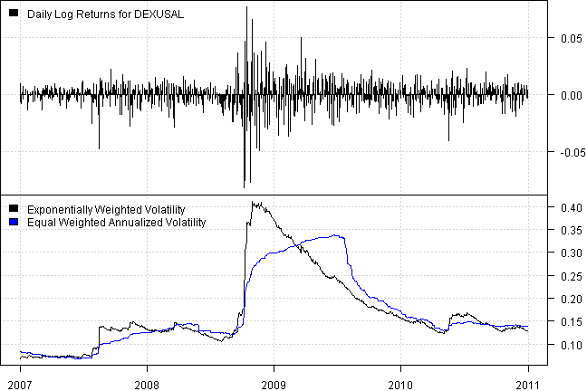
As expected, the Exponentially Weighted Volatility puts more weight on most recent observations and is a more reactive risk measure.
For your convenience, the 2016-04-10-Exponentially-Weighted-Volatility-RCPP post source code.