Thinking in SIT
20 Nov 2014To install Systematic Investor Toolbox (SIT) please visit About page.
The best way to understand how SIT works, in my opinion, is to do a side by side strategy test in Excel and one using SIT.
Let’s do step by step in investigating following simple strategy:
- allocate 50% to Stock if it’s prices is above 20 day moving average
- allocate 50% to Bond if it’s prices is above 20 day moving average
To code this strategy in Excel, we for example can downloaded historical prices for SPY and TLT. For simplicity, I generated in columns B and C Stock and Bond time series. To simulate each asset i used:
- Stock: 10% return and 20% volatility
- Bond: 4% return and 2% volatility
Next create columns D and E to hold 20 period moving averages for Stock and Bond. I.e. the formula in column D is D21 =AVERAGE(B2:B21) and in column E is E21 = AVERAGE(C2:C21)
Next create columns F and G to hold signals. I.e. F21 = IF(B21>D21,0.5,0) and G21 = IF(C21>E21,0.5,0)
To run back-test, we also need to compute asset returns, let column H and I hold Stock and Bond returns. I.e. H3 =B3/B2-1 and I3 = C3/C2-1
Finally store strategy returns in column J. I.e. J21 = F21H21+G21I21 (RET = W.Stock * RET.Stock + W.Bond * RET.Bond) and convert strategy returns into levels in column K. I.e. K3 = K2*(1+J3)
Let’s for the moment think that Excel is one big matrix, in this case:
- columns B and C hold asset’s prices
- columns D and E hold asset’s 20 day moving averages
- columns F and G hold asset’s signal. I.e. allocate 50% if prices > 20 day moving average
- columns H and I hold asset’s returns
- column J holds strategy’s return: RET = W.Stock * RET.Stock + W.Bond * RET.Bond
- column K holds strategy’s price
To convert this matrix into SIT, we need:
- download historical prices for SPY and TLT and align them so that dates on both series match
- compute 20 day moving averages for both assets
- compute signal: allocate 50%, if price > 20 day moving average
- compute strategy’s returns
Load historical data for SPY and TLT, and align it, so that dates on both time series match. We also adjust data for stock splits and dividends.
#*****************************************************************
# Load historical data
#*****************************************************************
library(SIT)
load.packages('quantmod')
tickers = spl('SPY,TLT')

data <- new.env()
getSymbols(tickers, src = 'yahoo', from = '1970-01-01', env = data, auto.assign = T)
for(i in ls(data)) data[[i]] = adjustOHLC(data[[i]], use.Adjusted=T)
bt.prep(data, align='remove.na')
Next let’s compute 20 day moving averages and signals. Please note that we are working with matrices below, so all computations are done for both time series with just single statement.
prices = data$prices
sma = bt.apply.matrix(prices, SMA, 20)
signal = iif(prices > sma, 0.5, 0)
Now we ready to back-test our strategy:
#*****************************************************************
# Code Strategies
#*****************************************************************
models = list()

data$weight[] = NA
data$weight[] = signal
models$strategy = bt.run.share(data, clean.signal=F, silent=T)
Finally create report:
#*****************************************************************
# Create Report
#*****************************************************************
plotbt(models, plotX = T, log = 'y', LeftMargin = 3, main = NULL)
mtext('Cumulative Performance', side = 2, line = 1)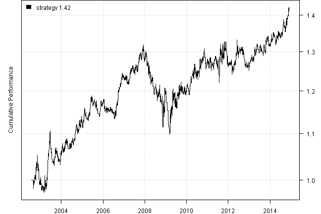
print(plotbt.strategy.sidebyside(models, make.plot=F, return.table=T))| strategy | |
|---|---|
| Period | Jul2002 - Dec2014 |
| Cagr | 2.87 |
| Sharpe | 0.45 |
| DVR | 0.37 |
| Volatility | 6.87 |
| MaxDD | -16.72 |
| AvgDD | -1.48 |
| VaR | -0.69 |
| CVaR | -1.01 |
| Exposure | 88.66 |
Ok we done.
So what is easier Excel worksheet or R back-test, both take some time to get used to. However, in the long run, R back-test will save you time because if you want to re-run it another day, you don’t need to worry about updating data and recalling strategy rules.
The data is auto update and adjusted. The strategy rules are stored in code with your own comments.
Another Example
Dan at Theta Trend posted a great example and tutorial on backtesting system in Excel. Please read Dan’s post at Backtesting A Basic ETF Rotation System in Excel Free Download
Let’s see how this strategy can be backtested using SIT:
#*****************************************************************
# Load historical data
#*****************************************************************
load.packages('quantmod')

tickers = '
    SPY, # S&P 500
    GLD, # Gold
    IEF, # 10 Year Treasury
    IYR, # US Real Estate
    EEM, # Emerging Markets
'

data <- new.env()
getSymbols.extra(tickers, src = 'yahoo', from = '1970-01-01', env = data, auto.assign = T)
for(i in ls(data)) data[[i]] = adjustOHLC(data[[i]], use.Adjusted=T)
bt.prep(data, align='remove.na')

#*****************************************************************
# Code Strategies
#*****************************************************************
prices = data$prices
n = ncol(prices)
month.ends = endpoints(prices, 'months')

plota.matplot(scale.one(prices))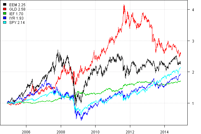
models = list()

#*****************************************************************
# Code Strategies, SPY - Buy & Hold
#*****************************************************************
data$weight[] = NA
data$weight$SPY = 1
models$SPY = bt.run.share(data, clean.signal=T, silent=T)

#*****************************************************************
# Code Strategies, Equal Weight, re-balanced monthly
#*****************************************************************
data$weight[] = NA
data$weight[month.ends,] = ntop(prices, n)[month.ends,]
models$equal.weight = bt.run.share(data, clean.signal=F, silent=T)

#*****************************************************************
# Code Strategies, Top 1 based on 5 month momentum, re-balanced monthly
#*****************************************************************
position.score = prices / mlag(prices, 5*21)

data$weight[] = NA
data$weight[month.ends,] = ntop(position.score[month.ends,], 1)
models$top1 = bt.run.share(data, trade.summary=T, clean.signal=F, silent=T)


#*****************************************************************
# Create Report
#*****************************************************************
plotbt(models, plotX = T, log = 'y', LeftMargin = 3, main = NULL)
mtext('Cumulative Performance', side = 2, line = 1)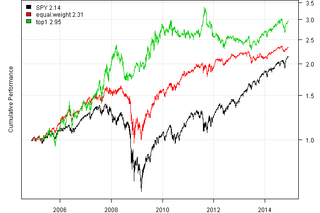
print(plotbt.strategy.sidebyside(models, make.plot=F, return.table=T))| SPY | equal.weight | top1 | |
|---|---|---|---|
| Period | Nov2004 - Dec2014 | Nov2004 - Dec2014 | Nov2004 - Dec2014 |
| Cagr | 7.88 | 8.69 | 11.36 |
| Sharpe | 0.48 | 0.59 | 0.62 |
| DVR | 0.24 | 0.52 | 0.49 |
| Volatility | 20.27 | 16.36 | 21.01 |
| MaxDD | -55.19 | -40.72 | -32.21 |
| AvgDD | -1.87 | -1.9 | -4.4 |
| VaR | -1.9 | -1.51 | -2.25 |
| CVaR | -3.13 | -2.46 | -3.14 |
| Exposure | 99.96 | 99.68 | 95.57 |
print(last.trades(models$top1, make.plot=F, return.table=T))| symbol | weight | entry.date | exit.date | entry.price | exit.price | return |
|---|---|---|---|---|---|---|
| IYR | 100 | 2013-04-30 | 2013-05-31 | 69.40 | 64.89 | -6.50 |
| SPY | 100 | 2013-05-31 | 2013-06-28 | 158.71 | 156.59 | -1.34 |
| SPY | 100 | 2013-06-28 | 2013-07-31 | 156.59 | 164.68 | 5.17 |
| SPY | 100 | 2013-07-31 | 2013-08-30 | 164.68 | 159.75 | -3.00 |
| SPY | 100 | 2013-08-30 | 2013-09-30 | 159.75 | 164.80 | 3.16 |
| SPY | 100 | 2013-09-30 | 2013-10-31 | 164.80 | 172.43 | 4.63 |
| SPY | 100 | 2013-10-31 | 2013-11-29 | 172.43 | 177.54 | 2.96 |
| SPY | 100 | 2013-11-29 | 2013-12-31 | 177.54 | 182.15 | 2.59 |
| SPY | 100 | 2013-12-31 | 2014-01-31 | 182.15 | 175.73 | -3.52 |
| SPY | 100 | 2014-01-31 | 2014-02-28 | 175.73 | 183.72 | 4.55 |
| SPY | 100 | 2014-02-28 | 2014-03-31 | 183.72 | 185.25 | 0.83 |
| SPY | 100 | 2014-03-31 | 2014-04-30 | 185.25 | 186.54 | 0.70 |
| IYR | 100 | 2014-04-30 | 2014-05-30 | 68.52 | 70.43 | 2.79 |
| IYR | 100 | 2014-05-30 | 2014-06-30 | 70.43 | 71.14 | 1.01 |
| EEM | 100 | 2014-06-30 | 2014-07-31 | 43.23 | 43.82 | 1.36 |
| EEM | 100 | 2014-07-31 | 2014-08-29 | 43.82 | 45.06 | 2.83 |
| IYR | 100 | 2014-08-29 | 2014-09-30 | 73.53 | 69.20 | -5.89 |
| SPY | 100 | 2014-09-30 | 2014-10-31 | 197.02 | 201.66 | 2.36 |
| IYR | 100 | 2014-10-31 | 2014-11-28 | 74.98 | 77.02 | 2.72 |
| IYR | 100 | 2014-11-28 | 2014-12-05 | 77.02 | 76.66 | -0.47 |
I think there is less chance of data error using SIT, and also update is automatic and takes no time on your part.
The key take away is to think about Excel operations as matrix operations to create a matrix with signals / allocations. This matrix with signals / allocations is used by SIT to create and display back-test(s).
(this report was produced on: 2014-12-07)