Walk Forward Optimization
24 Feb 2015To install Systematic Investor Toolbox (SIT) please visit About page.
There is an interesting article about Walk Forward Optimization at The Logical-Invest “Universal Investment Strategy”A Walk Forward Process on SPY and TLT
The strategy is based on the concept presented in the The SPY-TLT Universal Investment Strategy (UIS) article.
Below I will try to adapt a code from the posts:
#*****************************************************************
# Load historical data
#*****************************************************************
library(SIT)
load.packages('quantmod')

# load saved Proxies Raw Data, data.proxy.raw
# please see http://systematicinvestor.github.io/Data-Proxy/ for more details
load('data/data.proxy.raw.Rdata')

tickers = '
EQ = SPY + VFINX # S&P 500
FI = TLT + VUSTX # 20 Year Treasury
'

# uncomment if you want to use same data as in the source
#tickers = 'EQ=SPY, FI=TLT'

data <- new.env()
getSymbols.extra(tickers, src = 'yahoo', from = '1970-01-01', env = data, raw.data = data.proxy.raw, set.symbolnames = T, auto.assign = T)
  for(i in data$symbolnames) data[[i]] = adjustOHLC(data[[i]], use.Adjusted=T)
bt.prep(data, align='remove.na')

# Check data
plota.matplot(scale.one(data$prices),main='Asset Perfromance')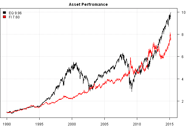
#*****************************************************************
# Setup
#*****************************************************************
prices = data$prices

frequency = 'months'
period.ends = endpoints(prices, frequency)
  period.ends = period.ends[period.ends > 0]

# all possible combinations
choices = expand.grid(
  EQ = seq(0, 100, by = 5),
  FI = seq(0, 100, by = 5),
KEEP.OUT.ATTRS=F)

# only select ones that sum up to 1
choices = choices[choices$EQ + choices$FI == 100,]
  choices = choices[sort.list(choices$EQ),]
  index = 1:nrow(choices)

# run back test over all combinations
result = rep.col(prices[,1], nrow(choices))
  colnames(result) = index

for(i in 1:nrow(choices)) {
  data$weight[] = NA
    data$weight$EQ[period.ends] = choices$EQ[i]/100
    data$weight$FI[period.ends] = choices$FI[i]/100
  model = bt.run.weight.fast(data)
  # uncomment if you want to get same results as in the source
  #model = bt.run.share(data, clean.signal=F, silent=T)
  result[,i] = model$equity
}

plota.matplot(result,main='Strategy Perfromance')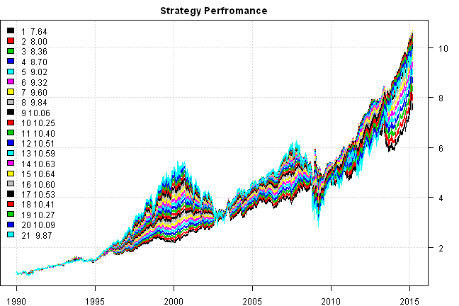
#*****************************************************************
# Pick Strategy based on modified Sharpe over 72 days
#*****************************************************************
sd.factor = 2.5
lookback.len = 72

lookback.return = (result / mlag(result,lookback.len))^(252/lookback.len) - 1

lookback.sd = bt.apply.matrix(result / mlag(result)-1, runSD, lookback.len)*sqrt(252)

mod.sharpe = lookback.return / lookback.sd ^ sd.factor
  mod.sharpe = mod.sharpe[period.ends,]

# pick best one
best.sharpe = ntop(mod.sharpe, 1)

# map back to original weights
weight = t(apply(best.sharpe, 1, function(x)
  colMeans(choices[index[x!=0],,drop=F])
)) / 100

weight = make.xts(weight, data$dates[period.ends])
#*****************************************************************
# Test strategy
#*****************************************************************
commission = list(cps = 0.01, fixed = 10.0, percentage = 0.0)

models = list()

data$weight[] = NA
	data$weight$EQ = 1
models$SP500 = bt.run.share(data, clean.signal=T, commission = commission, trade.summary=T, silent=T)


data$weight[] = NA
  data$weight[period.ends,] = as.matrix(weight)
models$UIS = bt.run.share(data, clean.signal=F, commission = commission, trade.summary=T, silent=T)


#*****************************************************************
# Create Report
#*****************************************************************
plotbt(models, plotX = T, log = 'y', LeftMargin = 3, main = NULL)
	mtext('Cumulative Performance', side = 2, line = 1)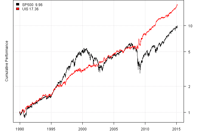
print(plotbt.strategy.sidebyside(models, make.plot=F, return.table=T, perfromance.fn=engineering.returns.kpi))| SP500 | UIS | |
|---|---|---|
| Period | Dec1989 - Feb2015 | Dec1989 - Feb2015 |
| Cagr | 9.54 | 11.98 |
| Sharpe | 0.59 | 1.21 |
| DVR | 0.48 | 1 |
| R2 | 0.81 | 0.82 |
| Volatility | 18.41 | 9.74 |
| MaxDD | -55.19 | -17.12 |
| Exposure | 99.98 | 98.83 |
| Win.Percent | 100 | 63.6 |
| Avg.Trade | 895.53 | 0.57 |
| Profit.Factor | NaN | 2.07 |
| Num.Trades | 1 | 533 |
print(last.trades(models$UIS, make.plot=F, return.table=T))| models$UIS | weight | entry.date | exit.date | nhold | entry.price | exit.price | return |
|---|---|---|---|---|---|---|---|
| EQ | 40 | 2014-04-30 | 2014-05-30 | 30 | 185.52 | 189.82 | 0.93 |
| FI | 60 | 2014-04-30 | 2014-05-30 | 30 | 108.71 | 111.92 | 1.77 |
| EQ | 50 | 2014-05-30 | 2014-06-30 | 31 | 189.82 | 193.74 | 1.03 |
| FI | 50 | 2014-05-30 | 2014-06-30 | 31 | 111.92 | 111.64 | -0.12 |
| EQ | 50 | 2014-06-30 | 2014-07-31 | 31 | 193.74 | 191.14 | -0.67 |
| FI | 50 | 2014-06-30 | 2014-07-31 | 31 | 111.64 | 112.38 | 0.33 |
| EQ | 60 | 2014-07-31 | 2014-08-29 | 29 | 191.14 | 198.68 | 2.37 |
| FI | 40 | 2014-07-31 | 2014-08-29 | 29 | 112.38 | 117.69 | 1.89 |
| EQ | 60 | 2014-08-29 | 2014-09-30 | 32 | 198.68 | 195.94 | -0.83 |
| FI | 40 | 2014-08-29 | 2014-09-30 | 32 | 117.69 | 115.21 | -0.84 |
| EQ | 50 | 2014-09-30 | 2014-10-31 | 31 | 195.94 | 200.55 | 1.18 |
| FI | 50 | 2014-09-30 | 2014-10-31 | 31 | 115.21 | 118.45 | 1.41 |
| EQ | 40 | 2014-10-31 | 2014-11-28 | 28 | 200.55 | 206.06 | 1.10 |
| FI | 60 | 2014-10-31 | 2014-11-28 | 28 | 118.45 | 121.96 | 1.78 |
| EQ | 45 | 2014-11-28 | 2014-12-31 | 33 | 206.06 | 205.54 | -0.11 |
| FI | 55 | 2014-11-28 | 2014-12-31 | 33 | 121.96 | 125.67 | 1.67 |
| EQ | 40 | 2014-12-31 | 2015-01-30 | 30 | 205.54 | 199.45 | -1.19 |
| FI | 60 | 2014-12-31 | 2015-01-30 | 30 | 125.67 | 138.00 | 5.89 |
| EQ | 50 | 2015-01-30 | 2015-02-26 | 27 | 199.45 | 211.38 | 2.99 |
| FI | 50 | 2015-01-30 | 2015-02-26 | 27 | 138.00 | 128.45 | -3.46 |
print(plotbt.monthly.table(models$UIS$equity, make.plot = F))| Jan | Feb | Mar | Apr | May | Jun | Jul | Aug | Sep | Oct | Nov | Dec | Year | MaxDD | |
|---|---|---|---|---|---|---|---|---|---|---|---|---|---|---|
| 1989 | 0.0 | 0.0 | ||||||||||||
| 1990 | 0.0 | 0.0 | -0.1 | -2.5 | 9.6 | 0.1 | 0.1 | -5.4 | 1.1 | 2.1 | 4.7 | 2.0 | 11.7 | -9.1 |
| 1991 | 1.4 | 2.1 | 0.9 | 0.7 | 1.5 | -3.0 | 1.4 | 3.6 | 1.6 | 0.2 | -0.8 | 6.7 | 17.3 | -4.6 |
| 1992 | -2.7 | 0.6 | -1.5 | 1.7 | 0.4 | 0.4 | 3.8 | 0.1 | 1.5 | -1.3 | 1.3 | 2.3 | 6.4 | -4.8 |
| 1993 | 0.3 | 1.3 | 1.8 | -1.3 | 0.7 | 3.1 | 1.4 | 4.1 | 0.2 | 1.0 | -1.7 | 0.9 | 12.2 | -4.1 |
| 1994 | 3.5 | -3.0 | -4.2 | 1.1 | 1.6 | -2.3 | 3.2 | 3.8 | -2.5 | 2.8 | -4.0 | 0.6 | 0.1 | -8.6 |
| 1995 | 2.5 | 2.9 | 1.4 | 2.4 | 5.2 | 1.4 | 0.6 | 1.1 | 3.6 | 0.0 | 3.5 | 2.2 | 30.2 | -2.8 |
| 1996 | 0.9 | -3.1 | 0.8 | 1.1 | 2.2 | 0.9 | -3.9 | -1.2 | 2.7 | 3.7 | 5.1 | -2.4 | 6.4 | -6.9 |
| 1997 | 1.4 | 0.4 | -3.9 | 6.0 | 1.9 | 3.1 | 5.3 | -2.7 | 2.8 | 3.1 | 1.4 | 1.7 | 22.1 | -8.8 |
| 1998 | 1.6 | 0.4 | 1.6 | 0.8 | -1.0 | 3.2 | -0.7 | 2.9 | 3.6 | -0.7 | 1.3 | 1.3 | 15.1 | -5.3 |
| 1999 | 1.8 | -4.3 | 1.6 | 2.3 | -2.1 | 3.8 | -3.0 | -0.5 | -2.3 | 0.2 | 1.6 | 1.8 | 0.6 | -11.3 |
| 2000 | -1.9 | 1.9 | 2.9 | -1.0 | -0.5 | 2.3 | 1.2 | 2.6 | -1.6 | 1.7 | 2.9 | 2.4 | 13.5 | -5.7 |
| 2001 | 0.6 | 0.0 | -1.1 | -2.5 | 0.2 | 0.8 | 0.8 | 0.9 | 0.9 | 5.0 | -4.5 | -1.6 | -0.9 | -9.1 |
| 2002 | 0.0 | -0.7 | 3.3 | -3.0 | 0.4 | 1.8 | 2.2 | 5.0 | 2.8 | -2.5 | 0.8 | 1.4 | 11.7 | -7.2 |
| 2003 | -1.2 | 1.7 | -1.0 | 2.9 | 6.1 | -1.0 | -5.3 | 1.8 | -1.1 | 5.3 | 0.8 | 3.4 | 12.7 | -11.2 |
| 2004 | 1.9 | 1.7 | -0.1 | -4.3 | 1.7 | 1.8 | -3.3 | 4.1 | 0.9 | 1.6 | 0.0 | 2.8 | 9.0 | -7.5 |
| 2005 | 0.3 | 0.3 | -1.1 | 3.8 | 3.1 | 1.8 | -1.2 | 1.0 | -1.2 | -2.4 | 4.4 | 0.3 | 9.3 | -5.2 |
| 2006 | 0.3 | 0.8 | -1.8 | 0.6 | -3.0 | 0.3 | 0.4 | 3.0 | 2.0 | 1.5 | 2.1 | -0.7 | 5.6 | -8.4 |
| 2007 | 0.5 | 0.2 | -0.6 | 3.2 | -0.3 | -1.3 | -2.5 | 1.7 | 0.6 | 1.7 | 3.0 | -0.8 | 5.3 | -6.5 |
| 2008 | -0.4 | -0.9 | 1.8 | -1.4 | -0.6 | -2.3 | -0.9 | 2.7 | 0.9 | -4.8 | 14.3 | 12.4 | 20.8 | -10.6 |
| 2009 | -12.4 | -3.4 | 4.6 | 9.9 | 5.8 | 0.2 | 5.0 | 3.2 | 3.1 | -2.3 | 3.7 | -2.2 | 14.3 | -15.6 |
| 2010 | -2.1 | 3.1 | 3.6 | 2.3 | -0.8 | 1.4 | 1.4 | 3.9 | 1.5 | -0.8 | -0.8 | 3.5 | 17.3 | -6.0 |
| 2011 | 1.2 | 3.2 | 0.0 | 2.6 | 1.1 | -2.1 | 1.2 | 4.3 | 6.1 | 2.1 | 1.0 | 2.3 | 25.5 | -3.5 |
| 2012 | 1.9 | 0.9 | -0.2 | 1.2 | -0.8 | 0.9 | 2.6 | 0.4 | 0.0 | -1.2 | 0.7 | -0.8 | 5.6 | -3.8 |
| 2013 | 0.1 | 1.2 | 2.1 | 3.0 | -1.8 | -2.1 | 4.0 | -3.0 | 3.2 | 4.6 | 1.8 | 1.0 | 14.7 | -6.3 |
| 2014 | -1.1 | 2.7 | 0.8 | 1.4 | 2.7 | 0.9 | -0.4 | 4.2 | -1.7 | 2.6 | 2.9 | 1.5 | 17.6 | -3.0 |
| 2015 | 4.7 | -0.5 | 4.2 | -2.1 | ||||||||||
| Avg | 0.1 | 0.4 | 0.5 | 1.2 | 1.3 | 0.6 | 0.5 | 1.7 | 1.1 | 0.9 | 1.8 | 1.7 | 11.4 | -6.6 |
plota(weight$EQ, type='s', main='SP500 Allocation in UIS Model')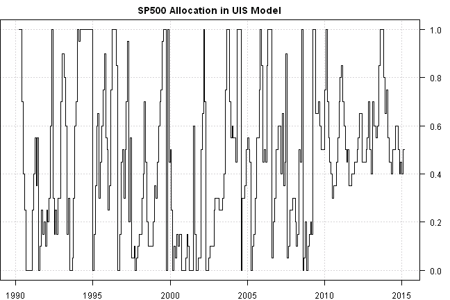
There a few more ideas you might try:
- select top N best performing combinations and average their weight
- do not consider portfolios with negative modified Sharpe
- if no portfolio is selected, invest into 100% TLT
It is very easy to modify code above to enforce these rules:
#*****************************************************************
# Modify strategy
#*****************************************************************
# 1. pick top 5
best.sharpe = ntop(mod.sharpe, 5)

  # 2. only consider portfolios with sharpe > 0
  best.sharpe = iif(mod.sharpe > 1, best.sharpe, 0)

# map back to original weights
weight = t(apply(best.sharpe, 1, function(x)
  colMeans(choices[index[x!=0],,drop=F])
)) / 100

weight = make.xts(weight, data$dates[period.ends])
  # 3. if no portfolio is selected, invest into 100% TLT
  weight = ifna(weight,0)
  weight$FI = weight$FI + 1 - rowSums(weight)


data$weight[] = NA
  data$weight[period.ends,] = as.matrix(weight)
models$UIS5 = bt.run.share(data, clean.signal=F, commission = commission, trade.summary=T, silent=T)


#*****************************************************************
# Create Report
#*****************************************************************
plotbt(models, plotX = T, log = 'y', LeftMargin = 3, main = NULL)
	mtext('Cumulative Performance', side = 2, line = 1)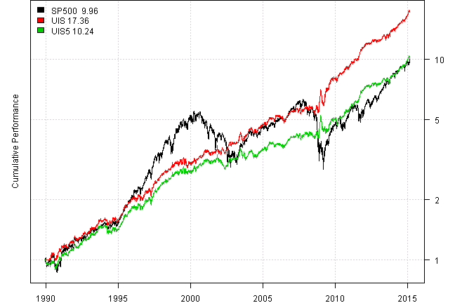
print(plotbt.strategy.sidebyside(models, make.plot=F, return.table=T, perfromance.fn=engineering.returns.kpi))| SP500 | UIS | UIS5 | |
|---|---|---|---|
| Period | Dec1989 - Feb2015 | Dec1989 - Feb2015 | Dec1989 - Feb2015 |
| Cagr | 9.54 | 11.98 | 9.66 |
| Sharpe | 0.59 | 1.21 | 1.03 |
| DVR | 0.48 | 1 | 0.9 |
| R2 | 0.81 | 0.82 | 0.88 |
| Volatility | 18.41 | 9.74 | 9.42 |
| MaxDD | -55.19 | -17.12 | -18.92 |
| Exposure | 99.98 | 98.83 | 99.83 |
| Win.Percent | 100 | 63.6 | 61.23 |
| Avg.Trade | 895.53 | 0.57 | 0.44 |
| Profit.Factor | NaN | 2.07 | 1.83 |
| Num.Trades | 1 | 533 | 570 |
Unfortunately, the performance is not reflected in our modifications. Another idea we might try was mentioned in the comment of original article by CyTrader, to to make lookback period and the F-Factor adaptive, for example:
- lookback can be in 2-6 months range
- F-Factor can be in 1.5-3.5 range
#*****************************************************************
# make lookback period and the F-Factor adaptive
#*****************************************************************
lookbacks = round(21 * seq(2, 6, by = 0.5))  # 2-6 months range
ffactors  = seq(1.5, 3.5, by = 0.5) # 1.5-3.5 range

# best sharpe across all parameters
best.weight = weight
  best.weight[] = 0
# average of best sharpes for each parameter
avg.weight = weight
  avg.weight[] = 0
best.mod.sharpe = rep(-10e10, nrow(weight))

for(lookback.len in lookbacks) {
  lookback.return = (result / mlag(result,lookback.len))^(252/lookback.len) - 1
  lookback.sd = bt.apply.matrix(result / mlag(result)-1, runSD, lookback.len)*sqrt(252)

  for(sd.factor in ffactors) {
    mod.sharpe = lookback.return / lookback.sd ^ sd.factor
      mod.sharpe = mod.sharpe[period.ends,]

    best.sharpe = ntop(mod.sharpe, 1)

    # map back to original weights
    iweight = t(apply(best.sharpe, 1, function(x)
      colMeans(choices[index[x!=0],,drop=F])
    )) / 100

    ibest.mod.sharpe = rowSums(best.sharpe * mod.sharpe)

    avg.weight = avg.weight +  iweight

    select.index =  ifna(ibest.mod.sharpe > best.mod.sharpe, F)
    best.mod.sharpe[select.index] = ibest.mod.sharpe[select.index]
    best.weight[select.index,] = iweight[select.index,]
  }
}

avg.weight = avg.weight / rowSums(avg.weight)
best.weight = best.weight / rowSums(best.weight)

data$weight[] = NA
  data$weight[period.ends,] = as.matrix(avg.weight)
models$UIS.A = bt.run.share(data, clean.signal=F, commission = commission, trade.summary=T, silent=T)


data$weight[] = NA
  data$weight[period.ends,] = as.matrix(best.weight)
models$UIS.B = bt.run.share(data, clean.signal=F, commission = commission, trade.summary=T, silent=T)


#*****************************************************************
# Create Report
#*****************************************************************
plotbt(models, plotX = T, log = 'y', LeftMargin = 3, main = NULL)
	mtext('Cumulative Performance', side = 2, line = 1)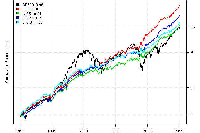
print(plotbt.strategy.sidebyside(models, make.plot=F, return.table=T, perfromance.fn=engineering.returns.kpi))| SP500 | UIS | UIS5 | UIS.A | UIS.B | |
|---|---|---|---|---|---|
| Period | Dec1989 - Feb2015 | Dec1989 - Feb2015 | Dec1989 - Feb2015 | Dec1989 - Feb2015 | Dec1989 - Feb2015 |
| Cagr | 9.54 | 11.98 | 9.66 | 10.79 | 9.99 |
| Sharpe | 0.59 | 1.21 | 1.03 | 1.16 | 1.13 |
| DVR | 0.48 | 1 | 0.9 | 0.99 | 1.03 |
| R2 | 0.81 | 0.82 | 0.88 | 0.86 | 0.9 |
| Volatility | 18.41 | 9.74 | 9.42 | 9.22 | 8.74 |
| MaxDD | -55.19 | -17.12 | -18.92 | -16.73 | -17.94 |
| Exposure | 99.98 | 98.83 | 99.83 | 97.84 | 99.18 |
| Win.Percent | 100 | 63.6 | 61.23 | 61.99 | 62.26 |
| Avg.Trade | 895.53 | 0.57 | 0.44 | 0.47 | 0.45 |
| Profit.Factor | NaN | 2.07 | 1.83 | 1.94 | 1.87 |
| Num.Trades | 1 | 533 | 570 | 584 | 575 |
gregor mentioned in his comment that simple monthly switching, based on prior three months returns, works quite well.
# simple monthly switching, based on prior three month returns, works well
position.score = prices / mlag(prices, 3 * 21)

data$weight[] = NA
	data$weight[period.ends,] = ntop(position.score[period.ends,], 1)
models$TOP.3M = bt.run.share(data, clean.signal=F, commission = commission, trade.summary=T, silent=T)

plotbt(models, plotX = T, log = 'y', LeftMargin = 3, main = NULL)
	mtext('Cumulative Performance', side = 2, line = 1)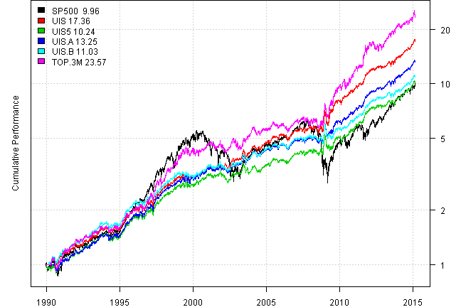
print(plotbt.strategy.sidebyside(models, make.plot=F, return.table=T, perfromance.fn=engineering.returns.kpi))| SP500 | UIS | UIS5 | UIS.A | UIS.B | TOP.3M | |
|---|---|---|---|---|---|---|
| Period | Dec1989 - Feb2015 | Dec1989 - Feb2015 | Dec1989 - Feb2015 | Dec1989 - Feb2015 | Dec1989 - Feb2015 | Dec1989 - Feb2015 |
| Cagr | 9.54 | 11.98 | 9.66 | 10.79 | 9.99 | 13.35 |
| Sharpe | 0.59 | 1.21 | 1.03 | 1.16 | 1.13 | 0.98 |
| DVR | 0.48 | 1 | 0.9 | 0.99 | 1.03 | 0.75 |
| R2 | 0.81 | 0.82 | 0.88 | 0.86 | 0.9 | 0.76 |
| Volatility | 18.41 | 9.74 | 9.42 | 9.22 | 8.74 | 13.71 |
| MaxDD | -55.19 | -17.12 | -18.92 | -16.73 | -17.94 | -17.08 |
| Exposure | 99.98 | 98.83 | 99.83 | 97.84 | 99.18 | 98.83 |
| Win.Percent | 100 | 63.6 | 61.23 | 61.99 | 62.26 | 66.78 |
| Avg.Trade | 895.53 | 0.57 | 0.44 | 0.47 | 0.45 | 1.16 |
| Profit.Factor | NaN | 2.07 | 1.83 | 1.94 | 1.87 | 2.36 |
| Num.Trades | 1 | 533 | 570 | 584 | 575 | 295 |
Let’s quickly check if other look back work equally well:
test.models = list()

for(i in 1:12) {
	position.score = prices / mlag(prices, i * 21)

	data$weight[] = NA
		data$weight[period.ends,] = ntop(position.score[period.ends,], 1)
	test.models[[paste0('TOP.', i, 'M')]] = bt.run.share(data, clean.signal=F, commission = commission, trade.summary=T, silent=T)
}

stats = plotbt.strategy.sidebyside(test.models, make.plot=F, return.table=T, perfromance.fn=engineering.returns.kpi)
performance.barchart.helper(stats, 'Sharpe,Cagr,Win.Percent,MaxDD,Volatility,Profit.Factor', c(T,T,T,T,F,T), sort.performance = F)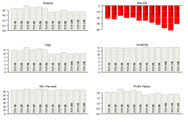
Looks like three months is the best look back period.
(this report was produced on: 2015-02-27)