Timing Luck
02 Jan 2015To install Systematic Investor Toolbox (SIT) please visit About page.
There are numerous articles talking about timing luck:
- Luck: The Difference Between Hired or Fired
- The Luck of the Rebalance Timing
- Timing Misfortune Strikes Again: 2013 Ivy10 Portfolio Performance
- Setting Expectations for Monthly Trading Systems
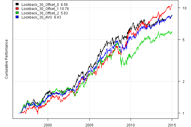
Let’s test concept of trading on different dates by simulating a momentum strategy with various lookbacks that trades on Quarter ends, and compare it to trading with 1/2 months offsets. I.e. let’s simulate trading on the second or third month of the quarter instead of the first month.
Load historical data.
#*****************************************************************
# Load historical data
#*****************************************************************
library(SIT)
load.packages('quantmod')
tickers = spl('DBC,EEM,EWJ,GLD,ICF,IEF,IEV,RWX,TLT,VTI')

data <- new.env()
getSymbols(tickers, src = 'yahoo', from = '1970-01-01', env = data, auto.assign = T)
  extend.data.proxy(data)
  for(i in ls(data)) data[[i]] = adjustOHLC(data[[i]], use.Adjusted=T)
bt.prep(data, align='remove.na')
Let’s define our test strategy:
test.strategy <- function(data, period.ends,
	top.n = 3,      # number of momentum positions
	lookback = 250,   # length of momentum look back
	lag = 1
){
	prices = coredata(data$prices)
	momentum = (mlag(prices, lag) / mlag(prices, (lookback + lag)) - 1)

	data$weight[] = NA
		data$weight[period.ends,] = ntop(momentum[period.ends,],top.n)
	data$weight
}
Now we ready to back-test our strategy:
#*****************************************************************
# Code Strategies
#*****************************************************************
prices = data$prices

models = list()

period.ends.high = endpoints(prices, 'months')
	n.period.ends = len(period.ends.high)

n.high.in.low = 12	# i.e. there are 12 months in 1 year
period.ends.low = endpoints(prices, 'years')

period.ends.low = endpoints(prices, 'quarters')
n.high.in.low = 3	# i.e. there are 3 months in 1 quater

pe = list()
pe[[1]] = which(!is.na( match(period.ends.high, period.ends.low) ))
for (i in 2:n.high.in.low) {
	pe[[i]] = pe[[(i-1)]] + 1
	pe[[i]] = iif(pe[[i]] > n.period.ends, n.period.ends, pe[[i]])
}

#*****************************************************************
# Code Strategies
#******************************************************************
lookbacks = c(30,120,250)
for (lookback in lookbacks) {
	weights = ifna(0 * data$weight, 0)
 for (i in 1:n.high.in.low) {
 	period.offset = i - 1
		weight = test.strategy(data, period.ends = period.ends.high[ pe[[i]] ], lookback = lookback)

		data$weight[] = weight
		models[[paste0('Lookback_', lookback, '_Offset_', period.offset)]] = bt.run.share(data, clean.signal=F, silent=T)

			weights = weights + bt.apply.matrix(weight, ifna.prev)/n.high.in.low
		}
	data$weight[] = weights
	models[[paste0('Lookback_',lookback,'_AVG')]] = bt.run.share(data, clean.signal=T, silent=T)
}

#*****************************************************************
# Report
#******************************************************************
for (lookback in lookbacks) {
	print('Lookback', lookback)
	models1 = models[grep(paste0('_', lookback, '_'), names(models))]

	plotbt(models1, plotX = T, log = 'y', LeftMargin = 3, main = NULL)
		mtext('Cumulative Performance', side = 2, line = 1)

	print(plotbt.strategy.sidebyside(models1, make.plot=F, return.table=T))
}
Lookback 30
| Lookback_30_Offset_0 | Lookback_30_Offset_1 | Lookback_30_Offset_2 | Lookback_30_AVG | |
|---|---|---|---|---|
| Period | Jun1996 - Jan2015 | Jun1996 - Jan2015 | Jun1996 - Jan2015 | Jun1996 - Jan2015 |
| Cagr | 12.29 | 13.69 | 9.99 | 12.2 |
| Sharpe | 0.91 | 0.95 | 0.78 | 1.02 |
| DVR | 0.86 | 0.83 | 0.71 | 0.94 |
| Volatility | 13.92 | 14.9 | 13.67 | 12.17 |
| MaxDD | -19.47 | -20.08 | -42.42 | -23.47 |
| AvgDD | -2.49 | -2.33 | -2.33 | -1.9 |
| VaR | -1.41 | -1.45 | -1.31 | -1.22 |
| CVaR | -2.06 | -2.18 | -2.04 | -1.78 |
| Exposure | 98.61 | 98.11 | 99.04 | 99.04 |
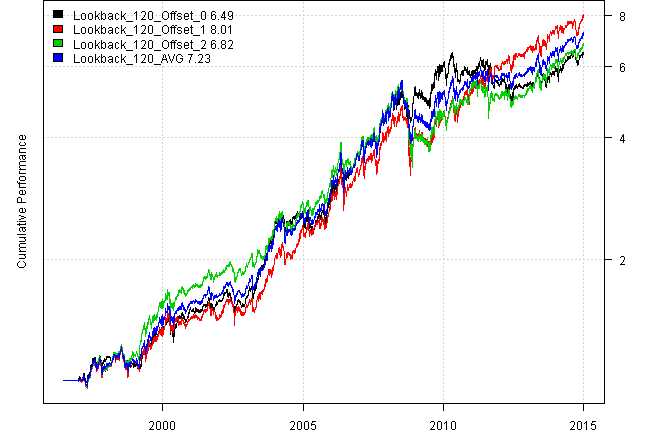
Lookback 120
| Lookback_120_Offset_0 | Lookback_120_Offset_1 | Lookback_120_Offset_2 | Lookback_120_AVG | |
|---|---|---|---|---|
| Period | Jun1996 - Jan2015 | Jun1996 - Jan2015 | Jun1996 - Jan2015 | Jun1996 - Jan2015 |
| Cagr | 10.62 | 11.88 | 10.92 | 11.27 |
| Sharpe | 0.8 | 0.87 | 0.79 | 0.83 |
| DVR | 0.73 | 0.79 | 0.75 | 0.79 |
| Volatility | 14.13 | 14.36 | 14.76 | 14.3 |
| MaxDD | -25.41 | -33.05 | -37.72 | -30.33 |
| AvgDD | -2.79 | -2.6 | -2.55 | -2.6 |
| VaR | -1.46 | -1.45 | -1.49 | -1.49 |
| CVaR | -2.09 | -2.12 | -2.26 | -2.15 |
| Exposure | 97.28 | 96.81 | 96.39 | 97.28 |
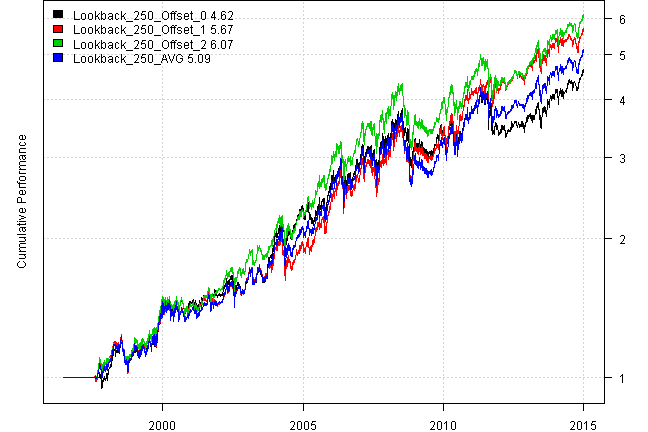
Lookback 250
| Lookback_250_Offset_0 | Lookback_250_Offset_1 | Lookback_250_Offset_2 | Lookback_250_AVG | |
|---|---|---|---|---|
| Period | Jun1996 - Jan2015 | Jun1996 - Jan2015 | Jun1996 - Jan2015 | Jun1996 - Jan2015 |
| Cagr | 8.61 | 9.82 | 10.22 | 9.19 |
| Sharpe | 0.65 | 0.74 | 0.77 | 0.68 |
| DVR | 0.63 | 0.69 | 0.74 | 0.64 |
| Volatility | 14.38 | 14.23 | 14.1 | 14.8 |
| MaxDD | -25.49 | -24.85 | -27.84 | -30.29 |
| AvgDD | -2.83 | -2.93 | -2.77 | -2.96 |
| VaR | -1.5 | -1.48 | -1.47 | -1.59 |
| CVaR | -2.16 | -2.14 | -2.14 | -2.26 |
| Exposure | 93.24 | 94.13 | 93.7 | 94.13 |
Somehow, strategy with 2 month offset is most volatile and has largest draw-down.
(this report was produced on: 2015-01-03)