Sortino vs Omega ratios
02 Apr 2015To install Systematic Investor Toolbox (SIT) please visit About page.
Following is quick visual comparison of Omega ratio vs Sortino ratio
library(SIT)
load.packages('quantmod')

#*****************************************************************
# Helper functions
#*****************************************************************
sortino.ratio = function(R,MAR) {
	r = R[R < MAR]
	(mean(R) - MAR) / sqrt(sum((MAR - r)^2) / length(r) )
}

omega.ratio = function(R,MAR) {
	#sum(pmax(R - MAR, 0)) / sum(pmax(MAR - R, 0))
	r = R - MAR
	- sum(r[r > 0]) / sum(r[r < 0])
}

#*****************************************************************
# check: Omega has a value of 1 at the mean of the distribution
#*****************************************************************
R = rnorm(100)
MAR = mean(R)

print(list(Sortino = sortino.ratio(R, MAR), Omega = omega.ratio(R,MAR)))
$Sortino [1] 0 $Omega [1] 1
#*****************************************************************
# Plot Sortino vs Omega
# based on [R graph with two y-axes](http://robjhyndman.com/hyndsight/r-graph-with-two-y-axes/)
#*****************************************************************
plot.sortino.omega = function(R, main='') {
  x = quantile(R, c(0.05, 0.95))
  x = seq(x[1],x[2], length.out=100)

  par(mar=c(5,4,4,5))
  plot(x, sapply(x, function(y) sortino.ratio(R,y)), xlab='MAR', ylab='Sortino',
    main=paste('Sortino vs Omega', main), type='l', col='red')

  par(new=TRUE)
  plot(x, sapply(x, function(y) omega.ratio(R,y)), xaxt="n",yaxt="n",xlab="", ylab='', type='l', col='blue')

  axis(4)
  mtext('Omega',side=4,line=3)
  legend("topright",col=c('red','blue'),lty=1,legend=c('Sortino','Omega'), bty='n')
}

plot.sortino.omega(R, ' based on random data')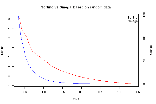
#*****************************************************************
# Load historical data
#*****************************************************************
data = env()
getSymbols('SPY', src = 'yahoo', from = '1970-01-01', env = data, auto.assign = T)

price = Ad(data$SPY)
ret = diff(log(price))

plot.sortino.omega(last(ret, 252), ' based on last year of SPY')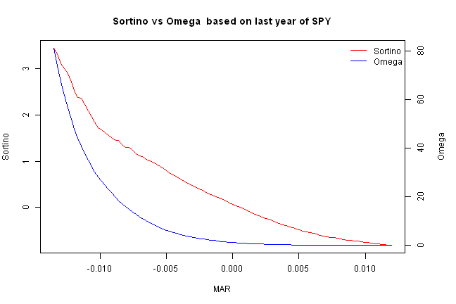
Re-run Maximizing Omega Ratio
Please set threshold used in Omega calculations (i.e. MAR) to a small number. Otherwise, optimizer will be forced to find corner solutions and result in not stable weights.
	#--------------------------------------------------------------------------
	# Create Efficient Frontier
	#--------------------------------------------------------------------------
	ia = aa.test.create.ia()
	n = ia$n

	# 0 <= x.i <= 0.8
	constraints = new.constraints(n, lb = 0, ub = 0.8)

	# SUM x.i = 1
	constraints = add.constraints(rep(1, n), 1, type = '=', constraints)

	# Omega - http://en.wikipedia.org/wiki/Omega_ratio
		# do not set threshold too high
		ia$parameters.omega = 1/100
		# convert annual to monthly
		ia$parameters.omega = ia$parameters.omega / 12

	max.omega.portfolio(ia, constraints)
[1] 0.000000e+00 7.255498e-02 1.688399e-01 1.097557e-16 0.000000e+00 [6] 2.661959e-01 0.000000e+00 4.924093e-01
	# create efficient frontier(s)
	ef.risk = portopt(ia, constraints, 50, 'Risk')

	#plot.ef(ia, list(ef.risk), portfolio.risk, T, T)


	# Plot Omega Efficient Frontiers and Transition Maps
	layout( matrix(1:4, nrow = 2, byrow=T) )

	# weights
	rownames(ef.risk$weight) = paste('Risk','weight',1:50,sep='_')
	plot.omega(ef.risk$weight[c(1,10,40,50), ], ia)

	# assets
	temp = diag(n)
	rownames(temp) = ia$symbols
	plot.omega(temp, ia)

	# portfolio
plot.ef(ia, list(ef.risk), portfolio.omega, T, T) 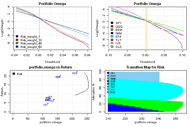
	#--------------------------------------------------------------------------
	# Create Efficient Frontier in Omega Ratio framework
	#--------------------------------------------------------------------------
	# Create maximum Omega Efficient Frontier
	ef.omega = portopt.omega(ia, constraints, 50)
i = 1 i = 2 i = 3 i = 4 i = 5 i = 6 i = 7 i = 8 i = 9 i = 10 i = 11 i = 12 i = 13 i = 14 i = 15 i = 16 i = 17 i = 18 i = 19 i = 20 i = 21 i = 22 i = 23 i = 24 i = 25 i = 26 i = 27 i = 28 i = 29 i = 30 i = 31 i = 32 i = 33 i = 34 i = 35 i = 36 i = 37 i = 38 i = 39 i = 40 i = 41 i = 42 i = 43 i = 44 i = 45 i = 46 i = 47 i = 48 i = 49 i = 50
	# Plot Omega Efficient Frontiers and Transition Maps
	layout( matrix(1:4, nrow = 2, byrow=T) )

	# weights
	plot.omega(ef.risk$weight[c(1,10,40,50), ], ia)
	#plot.omega(ef.omega$weight[c(1,10,40,50), ], ia)


	# weights
	rownames(ef.omega$weight) = paste('Omega','weight',1:50,sep='_')
	plot.omega(ef.omega$weight[c(1,10,40,50), ], ia)

	# portfolio
plot.ef(ia, list(ef.omega, ef.risk), portfolio.omega, T, T) 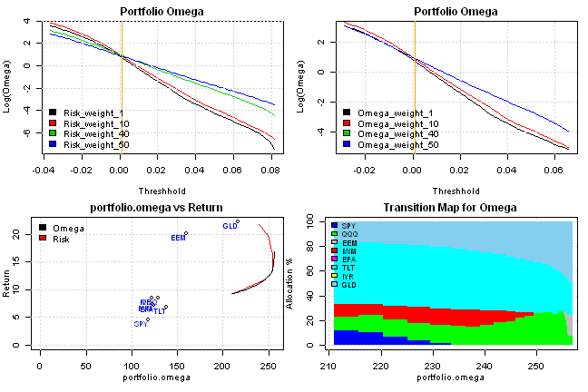
	#--------------------------------------------------------------------------
	# Compare Risk and Omega frontiers
	#--------------------------------------------------------------------------
	# Plot multiple Efficient Frontiers and Transition Maps
	layout( matrix(1:4, nrow = 2) )
	plot.ef(ia, list(ef.risk,ef.omega), portfolio.risk, F)
	plot.ef(ia, list(ef.risk,ef.omega), portfolio.omega, F)

	plot.transition.map(ef.risk)
	plot.transition.map(ef.omega)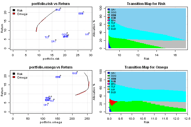
I will use methods presented in Optimizing Omega by H. Mausser, D. Saunders, L. Seco (2006) paper to construct optimal portfolios that maximize Omega Ratio.
#' @export
target.omega.portfolio <- function
(
	target.omega,
	type = 'mixed'
)
{
	target.omega = target.omega

	function
	(
		ia,			# input assumptions
		constraints	# constraints
	)
	{
		ia$parameters.omega = target.omega
		max.omega.portfolio(ia, constraints, type)
	}
}

#*****************************************************************
# Load historical data
#*****************************************************************
library(SIT)
load.packages('quantmod')

# load saved Proxies Raw Data, data.proxy.raw, to extend DBC and SHY
# please see http://systematicinvestor.github.io/Data-Proxy/ for more details
load('data/data.proxy.raw.Rdata')

tickers = '
LQD + VWESX
DBC + CRB
VTI +VTSMX # (or SPY)
ICF + VGSIX # (or IYR)
CASH = SHY + TB3Y
'

data <- new.env()
getSymbols.extra(tickers, src = 'yahoo', from = '1970-01-01', env = data, raw.data = data.proxy.raw, set.symbolnames = T, auto.assign = T)
for(i in data$symbolnames) data[[i]] = adjustOHLC(data[[i]], use.Adjusted=T)

#print(bt.start.dates(data))
bt.prep(data, align='remove.na', fill.gaps = T)


#*****************************************************************
# Code Strategies
#******************************************************************
obj = portfolio.allocation.helper(data$prices,
		periodicity = 'months', lookback.len = 60,
		min.risk.fns = list(
			EW=equal.weight.portfolio,
			RP=risk.parity.portfolio(),
			MD=max.div.portfolio,

			MV=min.var.portfolio,
			MVE=min.var.excel.portfolio,
			MO=target.omega.portfolio(0/100, 'lp'),

			MC=min.corr.portfolio,
			MCE=min.corr.excel.portfolio,
			MC2=min.corr2.portfolio,

			MS=max.sharpe.portfolio()
		),
		silent=T
)

commission = list(cps = 0.01, fixed = 10.0, percentage = 0.0)

models = create.strategies(obj, data, dates='1997::', commission=commission, silent=T)$models

#*****************************************************************
# Create Report
#*****************************************************************
#strategy.performance.snapshoot(models, T)
plotbt(models, plotX = T, log = 'y', LeftMargin = 3, main = NULL)
	mtext('Cumulative Performance', side = 2, line = 1)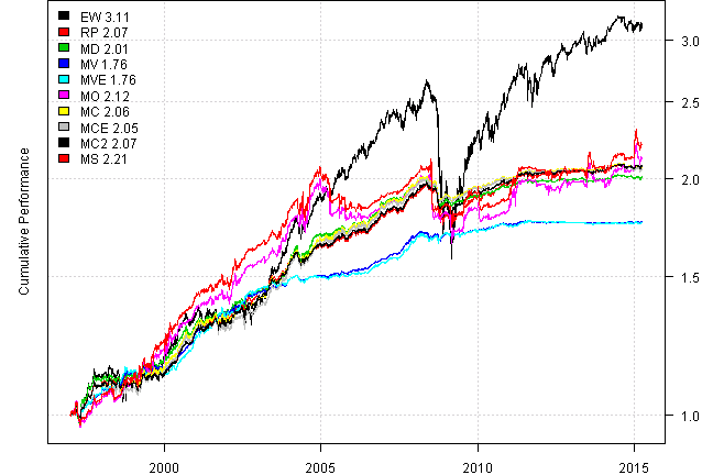
print(plotbt.strategy.sidebyside(models, make.plot=F, return.table=T, perfromance.fn=engineering.returns.kpi))| EW | RP | MD | MV | MVE | MO | MC | MCE | MC2 | MS | |
|---|---|---|---|---|---|---|---|---|---|---|
| Period | Jan1997 - Apr2015 | Jan1997 - Apr2015 | Jan1997 - Apr2015 | Jan1997 - Apr2015 | Jan1997 - Apr2015 | Jan1997 - Apr2015 | Jan1997 - Apr2015 | Jan1997 - Apr2015 | Jan1997 - Apr2015 | Jan1997 - Apr2015 |
| Cagr | 6.41 | 4.06 | 3.88 | 3.15 | 3.13 | 4.2 | 4.04 | 4.02 | 4.06 | 4.43 |
| Sharpe | 0.65 | 1.26 | 1.19 | 1.73 | 1.47 | 0.72 | 1.25 | 1.22 | 1.32 | 0.76 |
| DVR | 0.6 | 1.21 | 1.1 | 1.61 | 1.36 | 0.61 | 1.18 | 1.16 | 1.26 | 0.63 |
| R2 | 0.93 | 0.96 | 0.92 | 0.93 | 0.93 | 0.84 | 0.94 | 0.95 | 0.96 | 0.84 |
| Volatility | 10.51 | 3.2 | 3.26 | 1.8 | 2.12 | 5.95 | 3.21 | 3.27 | 3.07 | 5.99 |
| MaxDD | -40.68 | -12.11 | -8.74 | -2.88 | -2.97 | -19.4 | -7.97 | -7.57 | -8.67 | -17.97 |
| Exposure | 99.98 | 99.98 | 99.98 | 99.98 | 99.98 | 99.98 | 99.98 | 99.98 | 99.98 | 99.98 |
Now let’s do monthly
data = bt.change.periodicity(data, periodicity = 'months')


#*****************************************************************
# Code Strategies
#******************************************************************
obj = portfolio.allocation.helper(data$prices,
		periodicity = 'months', lookback.len = 24,
		min.risk.fns = list(
			EW=equal.weight.portfolio,
			RP=risk.parity.portfolio(),
			MD=max.div.portfolio,

			MV=min.var.portfolio,
			MVE=min.var.excel.portfolio,
			MO=target.omega.portfolio(0/100, 'lp'),

			MC=min.corr.portfolio,
			MCE=min.corr.excel.portfolio,
			MC2=min.corr2.portfolio,

			MS=max.sharpe.portfolio()
		),
		silent=T
)

models = create.strategies(obj, data, dates='1997::', commission=commission, silent=T)$models

#*****************************************************************
# Create Report
#*****************************************************************
#strategy.performance.snapshoot(models, T)
plotbt(models, plotX = T, log = 'y', LeftMargin = 3, main = NULL)
	mtext('Cumulative Performance', side = 2, line = 1)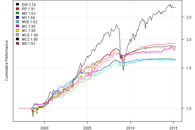
print(plotbt.strategy.sidebyside(models, make.plot=F, return.table=T, perfromance.fn=engineering.returns.kpi))| EW | RP | MD | MV | MVE | MO | MC | MCE | MC2 | MS | |
|---|---|---|---|---|---|---|---|---|---|---|
| Period | Jan1997 - Apr2015 | Jan1997 - Apr2015 | Jan1997 - Apr2015 | Jan1997 - Apr2015 | Jan1997 - Apr2015 | Jan1997 - Apr2015 | Jan1997 - Apr2015 | Jan1997 - Apr2015 | Jan1997 - Apr2015 | Jan1997 - Apr2015 |
| Cagr | 5.71 | 3.63 | 2.73 | 2.74 | 2.68 | 3.29 | 3.28 | 3.28 | 3.47 | 3.38 |
| Sharpe | 0.66 | 1.05 | 0.96 | 1.47 | 1.25 | 1.13 | 1.06 | 1.03 | 1.09 | 1.1 |
| DVR | 0.61 | 0.99 | 0.9 | 1.34 | 1.16 | 1.07 | 0.98 | 0.96 | 1.02 | 1.03 |
| R2 | 0.93 | 0.94 | 0.94 | 0.91 | 0.93 | 0.94 | 0.93 | 0.93 | 0.93 | 0.94 |
| Volatility | 8.97 | 3.44 | 2.83 | 1.84 | 2.12 | 2.88 | 3.08 | 3.15 | 3.16 | 3.06 |
| MaxDD | -37.17 | -12.8 | -7.54 | -3.17 | -2.59 | -3.22 | -6.56 | -6.54 | -9.92 | -3.38 |
| Exposure | 91.82 | 91.82 | 91.82 | 91.82 | 91.82 | 91.82 | 91.82 | 91.82 | 91.82 | 91.82 |
(this report was produced on: 2015-04-10)