Robust Asset Allocation

24 Feb 2015

To install Systematic Investor Toolbox (SIT) please visit About page.

The Scott’s Investments posted a spread sheet with Robust Asset Allocation (RAA) strategy based on the Alpha Architect’s - Our Robust Asset Allocation (RAA) Solution

Below I will try to adapt a code from the posts:

#*****************************************************************
# Load historical data
#*****************************************************************
library(SIT)
load.packages('quantmod')

# load saved Proxies Raw Data, data.proxy.raw
# please see http://systematicinvestor.github.io/Data-Proxy/ for more details
load('data/data.proxy.raw.Rdata')

tickers = '
SP500 = SPY
EAFE = EFA + VDMIX + VGTSX

REIT = VNQ + VGSIX # Vanguard REIT
COM = DBC + CRB # PowerShares DB Commodity Index Tracking Fund

US.BOND = IEF + VFITX
#US.BOND = BND + VBMFX # Vanguard Total Bond Market

US.VAL = PRF # PowerShares FTSE RAFI US 1000
US.MOM = PDP # PowerShares DWA Momentum Portfolio

INT.VAL = GVAL # Cambria Global Value
INT.MOM = PIZ # PowerShares DWA Developed Markets Momentum Portfolio

CASH = BIL + TB3M # Money Market or SHY/BIL
'


data <- new.env()
getSymbols.extra(tickers, src = 'yahoo', from = '1970-01-01', env = data, raw.data = data.proxy.raw, set.symbolnames = T, auto.assign = T)

# convert to monthly, 1-month-year format, to match Fama/French factors
for(i in data$symbolnames) {
	temp = to.monthly(data[[i]], indexAt='endof')
	index(temp) = as.Date(format(index(temp), '%Y-%m-1'),'%Y-%m-%d')
	data[[i]] = temp
}	

#*****************************************************************
# Get Fama/French factors
#****************************************************************** 
download = T
factors = get.fama.french.data('10_Portfolios_Prior_12_2', 'months',download = download, clean = F)
	temp = factors[["Average Value Weighted Returns -- Monthly"]]$High
	temp = cumprod(1+temp/100)
data$US.MOM = extend.data(data$US.MOM, make.stock.xts(temp), scale=T)
	
factors = get.fama.french.data('Portfolios_Formed_on_BE-ME', 'months',download = download, clean = F)
	temp = factors[["Value Weighted Returns -- Monthly"]][,'Hi 10']
	temp = cumprod(1+temp/100)
data$US.VAL = extend.data(data$US.VAL, make.stock.xts(temp), scale=T)
	
factors = get.fama.french.data('Global_ex_US_25_Portfolios_ME_Prior_12_2', 'months',download = download, clean = F)
	temp = factors[["Average Value Weighted Returns -- Monthly"]]$Big.High
	temp[] = rowMeans(factors[["Average Value Weighted Returns -- Monthly"]][,spl('Big.3,Big.4,Big.High')])
	temp = cumprod(1+temp/100)
data$INT.MOM = extend.data(data$INT.MOM, make.stock.xts(temp), scale=T)

factors = get.fama.french.data('Global_ex_US_25_Portfolios_ME_BE-ME', 'months',download = download, clean = F)
	temp = factors[["Average Value Weighted Returns -- Monthly"]]$Big.High
	temp[] = rowMeans(factors[["Average Value Weighted Returns -- Monthly"]][,spl('Big.3,Big.4,Big.High')])
	temp = cumprod(1+temp/100)
data$INT.VAL = extend.data(data$INT.VAL, make.stock.xts(temp), scale=T)

data$REIT = extend.data(data$REIT, data.proxy.raw$NAREIT, scale=T)




for(i in data$symbolnames) data[[i]] = adjustOHLC(data[[i]], use.Adjusted=T)

#print(bt.start.dates(data))

bt.prep(data, align='remove.na')

# Check data
plota.matplot(scale.one(data$prices),main='Asset Perfromance')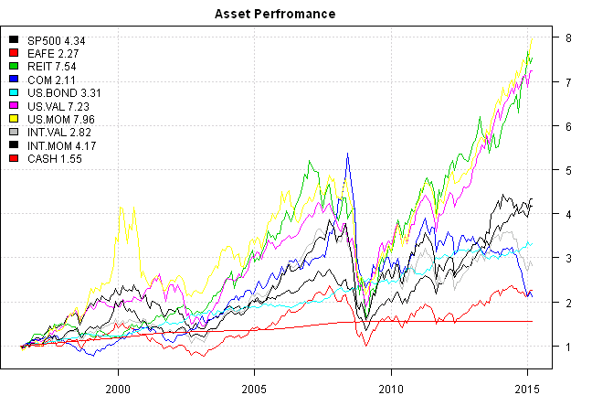

plot of chunk plot-2

#*****************************************************************
# Setup
#*****************************************************************
data$universe = data$prices > 0
	# do not allocate to CASH
	data$universe$CASH = NA

prices = data$prices * data$universe
	n = ncol(prices)
	nperiods = nrow(prices)

period.ends = endpoints(prices, 'months')
  period.ends = period.ends[period.ends > 0]

models = list()

#*****************************************************************
# Benchmarks
#*****************************************************************
data$weight[] = NA
	data$weight$SP500 = 1
models$SP500 = bt.run.share(data, clean.signal=T, trade.summary=T, silent=T)

data$weight[] = NA
	data$weight$SP500[period.ends,] = 0.5
	data$weight$US.BOND[period.ends,] = 0.5
models$S50.50 = bt.run.share(data, clean.signal=T, trade.summary=T, silent=T)

data$weight[] = NA
	data$weight$SP500[period.ends,] = 0.6
	data$weight$US.BOND[period.ends,] = 0.4
models$S60.40 = bt.run.share(data, clean.signal=T, trade.summary=T, silent=T)

#*****************************************************************
# IVY
# The [Quantitative Approach To Tactical Asset Allocation Strategy(QATAA) by Mebane T. Faber](http://mebfaber.com/timing-model/)
# [SSRN paper](http://papers.ssrn.com/sol3/papers.cfm?abstract_id=962461)
#*****************************************************************
sma = bt.apply.matrix(prices, SMA, 10)

# IVY5
prices1 = prices * NA
for(i in spl('SP500,EAFE,REIT,COM,US.BOND'))
	prices1[,i] = prices[,i]
	
nasset = sum(count(last(prices1)))

data$weight[] = NA
	data$weight[period.ends,] = ntop(prices1[period.ends,], nasset)
models$IVY5 = bt.run.share(data, clean.signal=F, trade.summary=T, silent=T)

# IVY5_MA
weight = NA * data$weight

weight = iif(prices1 > sma, 1/nasset, 0)
weight$CASH = 1 - rowSums(weight)

data$weight[] = NA
	data$weight[period.ends,] = weight[period.ends,]
models$IVY5_MA = bt.run.share(data, clean.signal=F, trade.summary=T, silent=T)

# IVY
nasset = sum(count(last(prices)))
data$weight[] = NA
	data$weight[period.ends,] = ntop(prices[period.ends,], n)
models$IVY = bt.run.share(data, clean.signal=F, trade.summary=T, silent=T)

# IVY_MA
weight = NA * data$weight

weight = iif(prices > sma, 1/nasset, 0)
weight$CASH = 1 - rowSums(weight)

data$weight[] = NA
	data$weight[period.ends,] = weight[period.ends,]
models$IVY_MA = bt.run.share(data, clean.signal=F, trade.summary=T, silent=T)

#*****************************************************************
# Strategy
# RAA_BAL = 40% Equity; 40% Real; 20% Bonds. Equity split between value and momentum. Risk-Managed.
# RAA_MOD = 60% Equity; 20% Real; 20% Bonds. Equity split between value and momentum. Risk-Managed.
# RAA_AGG = 80% Equity; 10% Real; 10% Bonds. Equity split between value and momentum. Risk-Managed.
#*****************************************************************
# RAA_MOD
target = list(
US.VAL = 60/4,
US.MOM = 60/4,
INT.VAL = 60/4,
INT.MOM = 60/4,
REIT = 20/2,
COM = 20/2,
US.BOND = 20
)

target.allocation = match(names(prices), toupper(names(target)))
	target.allocation = unlist(target)[target.allocation] / 100

	
	
sma = bt.apply.matrix(prices, SMA, 10)
	sma.signal = prices > sma
	sma.signal = ifna(sma.signal, F)

mom = prices / mlag(prices, 10) - 1
	mom.signal = mom > 0
	mom.signal = ifna(mom.signal, F)

# alternative
mom.cash = data$prices$CASH / mlag(data$prices$CASH, 12) - 1
	mom.signal = mom > as.vector(mom.cash)
	mom.signal = ifna(mom.signal, F)

weight = iif(sma.signal & mom.signal, 1, iif(sma.signal | mom.signal, 0.5, 0)) * rep.row(target.allocation, nperiods)
	weight = ifna(weight, 0)
weight$CASH = 1 - rowSums(weight)

data$weight[] = NA
	data$weight[period.ends,] = weight[period.ends,]
models$RAA = bt.run.share(data, clean.signal=F, trade.summary=T, silent=T)


print(last(weight[period.ends,], 24))

	REIT	COM	US.BOND	US.VAL	US.MOM	INT.VAL	INT.MOM	CASH
2013-04-01	0.10	0.05	0.2	0.15	0.15	0.150	0.150	0.050
2013-05-01	0.10	0.00	0.0	0.15	0.15	0.150	0.150	0.300
2013-06-01	0.10	0.00	0.0	0.15	0.15	0.150	0.150	0.300
2013-07-01	0.10	0.00	0.0	0.15	0.15	0.150	0.150	0.300
2013-08-01	0.05	0.00	0.0	0.15	0.15	0.150	0.150	0.350
2013-09-01	0.05	0.00	0.0	0.15	0.15	0.150	0.150	0.350
2013-10-01	0.10	0.00	0.0	0.15	0.15	0.150	0.150	0.300
2013-11-01	0.00	0.00	0.0	0.15	0.15	0.150	0.150	0.400
2013-12-01	0.00	0.00	0.0	0.15	0.15	0.150	0.150	0.400
2014-01-01	0.05	0.00	0.1	0.15	0.15	0.150	0.150	0.250
2014-02-01	0.05	0.05	0.1	0.15	0.15	0.150	0.150	0.200
2014-03-01	0.10	0.10	0.1	0.15	0.15	0.150	0.150	0.100
2014-04-01	0.10	0.10	0.2	0.15	0.15	0.150	0.150	0.000
2014-05-01	0.10	0.10	0.2	0.15	0.15	0.150	0.150	0.000
2014-06-01	0.10	0.05	0.2	0.15	0.15	0.150	0.150	0.050
2014-07-01	0.10	0.00	0.2	0.15	0.15	0.075	0.075	0.250
2014-08-01	0.10	0.00	0.2	0.15	0.15	0.000	0.075	0.325
2014-09-01	0.10	0.00	0.2	0.15	0.15	0.000	0.000	0.400
2014-10-01	0.10	0.00	0.2	0.15	0.15	0.000	0.000	0.400
2014-11-01	0.10	0.00	0.2	0.15	0.15	0.000	0.000	0.400
2014-12-01	0.10	0.00	0.2	0.15	0.15	0.000	0.000	0.400
2015-01-01	0.10	0.00	0.2	0.15	0.15	0.000	0.000	0.400
2015-02-01	0.10	0.00	0.2	0.15	0.15	0.000	0.075	0.325
2015-03-01	0.10	0.00	0.2	0.15	0.15	0.000	0.075	0.325

#*****************************************************************
# Report
#*****************************************************************
#strategy.performance.snapshoot(models, T)
plotbt(models, plotX = T, log = 'y', LeftMargin = 3, main = NULL)
	mtext('Cumulative Performance', side = 2, line = 1)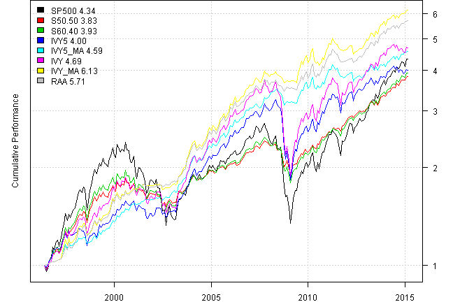

plot of chunk plot-2

print(plotbt.strategy.sidebyside(models, make.plot=F, return.table=T,perfromance.fn = engineering.returns.kpi))

	SP500	S50.50	S60.40	IVY5	IVY5_MA	IVY	IVY_MA	RAA
Period	Jun1996 - Mar2015	Jun1996 - Mar2015	Jun1996 - Mar2015	Jun1996 - Mar2015	Jun1996 - Mar2015	Jun1996 - Mar2015	Jun1996 - Mar2015	Jun1996 - Mar2015
Cagr	8.14	7.42	7.57	7.67	8.46	8.59	10.15	9.74
Sharpe	0.58	0.95	0.84	0.72	1.25	0.68	1.21	1.28
DVR	0.35	0.84	0.7	0.66	1.22	0.6	1.17	1.24
R2	0.6	0.88	0.83	0.91	0.97	0.88	0.97	0.97
Volatility	15.47	7.86	9.2	11.16	6.67	13.43	8.24	7.47
MaxDD	-50.79	-21.3	-27.81	-43.49	-11.21	-49.18	-11.17	-9.35
Exposure	99.56	99.56	99.56	99.56	99.56	99.56	99.56	99.56
Win.Percent	100	100	100	59.09	65.15	59.82	64.98	64.48
Avg.Trade	334.12	141.32	146.46	0.14	0.17	0.09	0.12	0.13
Profit.Factor	NaN	NaN	NaN	1.49	1.88	1.5	2.03	1.98
Num.Trades	1	2	2	1117	921	2016	1545	1354

layout(1)
barplot.with.labels(sapply(models, compute.turnover, data), 'Average Annual Portfolio Turnover')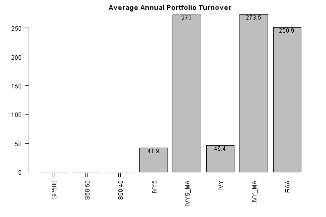

plot of chunk plot-2

(this report was produced on: 2015-03-19)

Systematic Investor's Blog About Contact

Robust Asset Allocation

Related Posts

RFinance 2016 15 May 2016

Benchmark Plus 14 Apr 2016

Exponentially Weighted Volatility using RCPP 10 Apr 2016