RSI and Random Forest
04 Nov 2014To install Systematic Investor Toolbox (SIT) please visit About page.
Tad Slaff at InovanceTech published How to Trade the RSI: An analysis using a Support Vector Machine post that I like. Below I will explore it a bit more.
Load Historical Prices. Let’s start with AUD/USD 4 hour bar pricesdropbox.
#*****************************************************************
# Load historical data
#******************************************************************
library(SIT)
load.packages('quantmod')

data <- new.env()
data$AUDUSD = read.xts('data/AUDUSD.csv', format='%m/%d/%y %H:%M', index.class = c("POSIXlt", "POSIXt"))
#plota(data$AUDUSD, type='l')
bt.prep(data, align='remove.na')
Create Indicators and Train SVM:
# helper functions
make.predictor <- function(x) { iif(x > 0, 1, -1) }

#*****************************************************************
# Code Strategies
#******************************************************************
load.packages('e1071,ggplot2')

indicators = as.xts(list(
RSI3 = RSI(Cl(data$AUDUSD), 3),
DEMA10 = DEMA(Cl(data$AUDUSD), 10),
CCI2 = CCI(HLC(data$AUDUSD), 20)
))

SMA50 = SMA(Op(data$AUDUSD), 50)

DataSet = as.xts(list(
RSI3 = RSI(Op(data$AUDUSD), 3),
Trend = Op(data$AUDUSD) - SMA50,
Direction = make.predictor(Cl(data$AUDUSD) - Op(data$AUDUSD))
))

# remove NA's
DataSet = DataSet[-(1:49),]

#Separate the data into 60% training set to build our model, 20% test set to
# test the patterns we found, and 20% validation set to run our strategy over new

Training = DataSet[1:4528,]
Test = DataSet[4529:6038,]
Val = DataSet[6039:7548,]

#Build our support vector machine using a radial basis function as our kernel, the cost, or C, at 1, and the gamma function at , or 1 over the number of inputs we are using

SVM = svm(Direction ~ RSI3 + Trend, data=Training, kernel="radial",cost=1,gamma=1/2)

#Run the algorithm once more over the training set to visualize the patterns it found
TrainingPredictions = predict(SVM,Training,type="class")
TrainingPredictions = make.predictor(TrainingPredictions)

# Plot
TrainingData = data.frame(Training,TrainingPredictions)
ggplot(TrainingData, aes(x=Trend,y=RSI3)) +
stat_density2d(geom="contour",aes(color=as.factor(TrainingPredictions)))+
labs(title="SVM RSI3 and Trend Predictions",
x="Open - SMA50",y="RSI3",color="Training Predictions")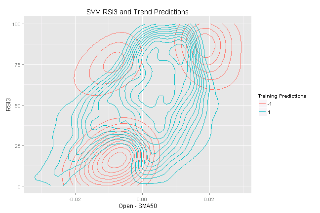
Now that we have found a basic set of rules that the SVM uncovered, lets test to see how well they hold up over new data, our test set.
# Now that we have found a basic set of rules that the SVM uncovered,
# lets test to see how well they hold up over new data, our test set.

ShortRange1 = Test$RSI3 < 25 & Test$Trend > -.010 & Test$Trend < -.005
ShortRange2 = Test$RSI3 > 70 & Test$Trend < -.005
ShortRange3 = Test$RSI3 > 75 & Test$Trend > .015

LongRange1 = Test$RSI3 < 25 & Test$Trend < -.02
LongRange2 = Test$RSI3 > 50 & Test$RSI3 < 75 & Test$Trend > .005 & Test$Trend < .01


# Now lets see how well these patterns hold up over out test set:
ShortTrades = Test[ShortRange1 | ShortRange2 | ShortRange3,]
ShortCorrect = sum(ShortTrades$Direction == -1)/nrow(ShortTrades)*100
ShortCorrect
[1] 57.82313
LongTrades  = Test[LongRange1 | LongRange2, ]
LongCorrect = sum(LongTrades$Direction == 1)/nrow(LongTrades)*100
LongCorrect
[1] 57.14286
Wow! 58% (85 correct out of 147 trades) for our short trades and 57% (80 correct out of 140 trades) for our long trades.
Now lets turn this into an actual trading strategy with a stop loss and take profit as our exit conditions.
(this report was produced on: 2014-12-07)