Quarterly Tactical Strategy
16 Feb 2015To install Systematic Investor Toolbox (SIT) please visit About page.
Another interesting post by QuantStrat TradeR: The Quarterly Tactical Strategy (aka QTS)
The Quarterly Tactical Strategy was published by Cliff Smith.
Below I will try to adapt a code from the post:
#*****************************************************************
# Load historical data
#*****************************************************************
library(SIT)
load.packages('quantmod')

tickers = '
US.SC = VB + NAESX # U.S. Small Cap
EM.BOND = VWOB + PREMX # Emerging Market Government Bond
EM.EQ = VWO + VEIEX # Emerging Markets
US.CORP.BOND = VCIT + VFICX # Intermediate Corporate Bond
US.MBS = VMBS + VFIIX # Mortgage-Backed Bonds
US.LC = SPY + VFINX # S&P 500
US.REIT = VNQ +  VGSIX # MSCI U.S. REIT
INTL.EQ = VEU + VGTSX # FTSE All-World ex-U.S.
CASH = TLT + VUSTX # Long-Tern Treasury
'

data <- new.env()
getSymbols.extra(tickers, src = 'yahoo', from = '1970-01-01', env = data, set.symbolnames = T, auto.assign = T)
for(i in data$symbolnames) data[[i]] = adjustOHLC(data[[i]], use.Adjusted=T)

#print(bt.start.dates(data))
bt.prep(data, align='remove.na', fill.gaps = T)

# Check data
plota.matplot(scale.one(data$prices),main='Asset Perfromance')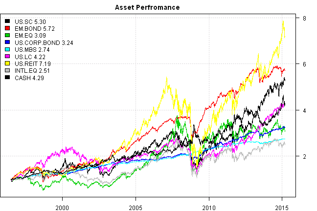
#*****************************************************************
# Setup
#*****************************************************************
data$universe = data$prices > 0
  # do not allocate to CASH, or BENCH
  data$universe$CASH = NA

prices = data$prices * data$universe
  n = ncol(prices)
  nperiods = nrow(prices)


frequency = 'quarters'
# find period ends, can be 'weeks', 'months', 'quarters', 'years'
period.ends = endpoints(prices, frequency)
  period.ends = period.ends[period.ends > 0]

models = list()

commission = list(cps = 0.01, fixed = 10.0, percentage = 0.0)

# lag prices by 1 day
#prices = mlag(prices)
#*****************************************************************
# Equal Weight each re-balancing period
#******************************************************************
data$weight[] = NA
  data$weight[period.ends,] = ntop(prices[period.ends,], n)
models$ew = bt.run.share(data, clean.signal=F, commission = commission, trade.summary=T, silent=T)

#*****************************************************************
# Strategy:
#
# Select the top-ranked asset each quarter based on
# 5-month and 20-day total returns weighted 50% each.
#
# A cash filter must be passed for the top-ranked mutual fund to be selected
# in any given period. The cash filter is the 3-month moving average.
#******************************************************************
mom.5m = prices / mlag(prices, 5*21) -1
mom.20d = prices / mlag(prices, 20) -1

# compute 3 month moving average
sma = bt.apply.matrix(prices, SMA, 3*21)

# go to cash if prices falls below 3 month moving average
go2cash = prices <= sma
  go2cash.d = ifna(go2cash, T)


# compute moving average in months
sma = bt.apply.matrix(prices, SMA, 3, periodicity='months')

go2cash = prices <= sma
  go2cash.m = ifna(go2cash, T)


# all logic below is done at period.ends
mom.5m = mom.5m[period.ends,]
mom.20d = mom.20d[period.ends,]
go2cash.d = go2cash.d[period.ends,]
go2cash.m = go2cash.m[period.ends,]

#*****************************************************************
# Rank total score
#*****************************************************************
# target allocation
target.allocation = ntop(0.5 * mom.5m + 0.5 * mom.20d ,1)

# If asset is above it's 3 month moving average it gets allocation
weight = iif(go2cash.d, 0, target.allocation)

# otherwise, it's weight is allocated to cash
weight$CASH = 1 - rowSums(weight)

data$weight[] = NA
  data$weight[period.ends,] = weight
models$QTS.d = bt.run.share(data, clean.signal=F, commission = commission, trade.summary=T, silent=T)


# same but using monthly moving average to trigger go to cash
weight = iif(go2cash.m, 0, target.allocation)
weight$CASH = 1 - rowSums(weight)

data$weight[] = NA
  data$weight[period.ends,] = weight
models$QTS.m = bt.run.share(data, clean.signal=F, commission = commission, trade.summary=T, silent=T)

#*****************************************************************
# Rank each component of total score first
#*****************************************************************
# target allocation
target.allocation[] = ntop(1.01 * bt.rank(mom.5m, F,T) + bt.rank(mom.20d, F,T) ,1)

# If asset is above it's 3 month moving average it gets allocation
weight = iif(go2cash.d, 0, target.allocation)

# otherwise, it's weight is allocated to cash
weight$CASH = 1 - rowSums(weight)

data$weight[] = NA
  data$weight[period.ends,] = weight
models$QTS.RANK.d = bt.run.share(data, clean.signal=F, commission = commission, trade.summary=T, silent=T)


# same but using monthly moving average to trigger go to cash
weight = iif(go2cash.m, 0, target.allocation)
weight$CASH = 1 - rowSums(weight)

data$weight[] = NA
  data$weight[period.ends,] = weight
models$QTS.RANK.m = bt.run.share(data, clean.signal=F, commission = commission, trade.summary=T, silent=T)

#*****************************************************************
# Report
#*****************************************************************
#strategy.performance.snapshoot(models, T)
plotbt(models, plotX = T, log = 'y', LeftMargin = 3, main = NULL)
	mtext('Cumulative Performance', side = 2, line = 1)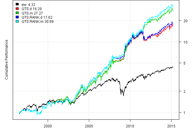
print(plotbt.strategy.sidebyside(models, make.plot=F, return.table=T))| ew | QTS.d | QTS.m | QTS.RANK.d | QTS.RANK.m | |
|---|---|---|---|---|---|
| Period | Jun1996 - Mar2015 | Jun1996 - Mar2015 | Jun1996 - Mar2015 | Jun1996 - Mar2015 | Jun1996 - Mar2015 |
| Cagr | 8.13 | 16.08 | 19.32 | 16.57 | 20.12 |
| Sharpe | 0.67 | 0.91 | 1.07 | 0.96 | 1.15 |
| DVR | 0.61 | 0.76 | 0.81 | 0.82 | 0.86 |
| Volatility | 12.89 | 18.28 | 17.99 | 17.54 | 17.32 |
| MaxDD | -44.61 | -26.78 | -26.78 | -25 | -19.39 |
| AvgDD | -1.55 | -3.09 | -3.01 | -2.87 | -2.77 |
| VaR | -1.16 | -1.79 | -1.75 | -1.71 | -1.69 |
| CVaR | -1.96 | -2.82 | -2.72 | -2.71 | -2.61 |
| Exposure | 99.98 | 99.98 | 99.98 | 99.98 | 99.98 |
Given that each quarter only one top fund is selected it is natural that strategy is sensitive to input parameters. However, the change in performance from go to cash rule based on 63 days vs 3 months is staggering.
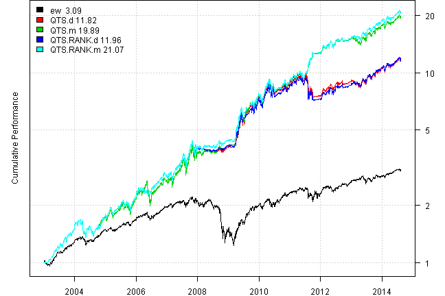
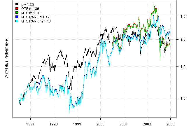
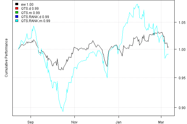
Finally, let’s zoom in on various periods:
dates.range = c('2002-12-31::2014-08-15', '::2002-12-31', '2014-08-15::')

for(dates in dates.range) {
models1 = bt.trim(models, dates=dates)
plotbt(models1, plotX = T, log = 'y', LeftMargin = 3, main = NULL)
	mtext('Cumulative Performance', side = 2, line = 1)
print(plotbt.strategy.sidebyside(models1, make.plot=F, return.table=T))
}
| ew | QTS.d | QTS.m | QTS.RANK.d | QTS.RANK.m | |
|---|---|---|---|---|---|
| Period | Dec2002 - Aug2014 | Dec2002 - Aug2014 | Dec2002 - Aug2014 | Dec2002 - Aug2014 | Dec2002 - Aug2014 |
| Cagr | 10.2 | 23.66 | 29.32 | 23.79 | 29.96 |
| Sharpe | 0.74 | 1.15 | 1.4 | 1.2 | 1.48 |
| DVR | 0.64 | 1.07 | 1.25 | 1.13 | 1.32 |
| Volatility | 14.5 | 20.3 | 19.86 | 19.34 | 19 |
| MaxDD | -44.61 | -25.99 | -25.99 | -25 | -19.13 |
| AvgDD | -1.43 | -2.89 | -2.79 | -2.61 | -2.49 |
| VaR | -1.36 | -2.06 | -1.98 | -1.86 | -1.81 |
| CVaR | -2.26 | -3.15 | -3.01 | -3.01 | -2.86 |
| Exposure | 100 | 100 | 100 | 100 | 100 |
| ew | QTS.d | QTS.m | QTS.RANK.d | QTS.RANK.m | |
|---|---|---|---|---|---|
| Period | Jun1996 - Dec2002 | Jul1996 - Dec2002 | Jul1996 - Dec2002 | Jul1996 - Dec2002 | Jul1996 - Dec2002 |
| Cagr | 5.18 | 5.19 | 5.11 | 6.27 | 6.2 |
| Sharpe | 0.56 | 0.43 | 0.42 | 0.51 | 0.5 |
| DVR | 0.4 | 0.32 | 0.32 | 0.41 | 0.41 |
| Volatility | 9.81 | 14.21 | 14.23 | 13.93 | 13.95 |
| MaxDD | -20.72 | -26.78 | -26.78 | -19.39 | -19.39 |
| AvgDD | -2.05 | -3.18 | -3.37 | -3.53 | -3.9 |
| VaR | -0.98 | -1.37 | -1.37 | -1.36 | -1.36 |
| CVaR | -1.43 | -2.15 | -2.15 | -2.11 | -2.11 |
| Exposure | 99.94 | 100 | 100 | 100 | 100 |
| ew | QTS.d | QTS.m | QTS.RANK.d | QTS.RANK.m | |
|---|---|---|---|---|---|
| Period | Aug2014 - Mar2015 | Aug2014 - Mar2015 | Aug2014 - Mar2015 | Aug2014 - Mar2015 | Aug2014 - Mar2015 |
| Cagr | 0.83 | -1.52 | -1.52 | -1.52 | -1.52 |
| Sharpe | 0.15 | -0.03 | -0.03 | -0.03 | -0.03 |
| DVR | 0.04 | -0.01 | -0.01 | -0.01 | -0.01 |
| Volatility | 8.15 | 15.71 | 15.71 | 15.71 | 15.71 |
| MaxDD | -5.29 | -14.33 | -14.33 | -14.33 | -14.33 |
| AvgDD | -1.03 | -3.38 | -3.38 | -3.38 | -3.38 |
| VaR | -0.89 | -1.94 | -1.94 | -1.94 | -1.94 |
| CVaR | -1.04 | -2.35 | -2.35 | -2.35 | -2.35 |
| Exposure | 100 | 100 | 100 | 100 | 100 |
(this report was produced on: 2015-03-12)