Optimizing Run Time for Large Universe
22 Apr 2015To install Systematic Investor Toolbox (SIT) please visit About page.
Recently, I was asked if Systematic Investor Toolbox (SIT) back-testing framework is suitable for running large universe back-tests.
Below, I will present the steps I took to test and optimize the running time. I will base this experiment on the Volatility Quantiles post i wrote back in 2012.
First, let’s generate 10 years of daily data for 25,000 securities.
Please note that this code requires lot’s of memory to store results;
hence, you might want to add --max-mem-size=8000M to your R parameters.
# https://systematicinvestor.wordpress.com/2012/06/05/volatility-quantiles/
#*****************************************************************
# Load historical data
#*****************************************************************
library(SIT)
load.packages('quantmod')

tic(11)

tic(1)

	n = 25 * 1000
	nperiods = 10 * 252

	# force high vol to small return
	library(MASS)
	mu = c(5,20) / 100
	sigma = c(5,10) / 100
	rho = -0.9
	cov.matrix = sigma%*%t(sigma) * matrix(c(1,rho,rho,1),2,2)
	temp = mvrnorm(n, mu, cov.matrix)

	mu = temp[,1]
	sigma = temp[,2]
		sigma[sigma < 1/100] = 1/100

	ret = matrix(rnorm(n*nperiods), nr=n)
		ret = t(ret * sigma/sqrt(252) + mu/252)

		#colnames(ret) = paste('A',1:n)
		dates = seq(Sys.Date()-nperiods+1, Sys.Date(), 1)
	#prices = bt.apply.matrix(1 + ret, cumprod)
	#plot(prices[,1])

	#data = env(
	#	symbolnames = colnames(prices)
	#	dates = dates
	#	fields = 'Cl'
	#	Cl = prices)
	#bt.prep.matrix(data)
Next I tried to run the original code from the Volatility Quantiles post and eventually run out of memory.
Below i modified original code to make it work.
    #*****************************************************************
    # Create Quantiles based on the historical one year volatility
    #******************************************************************
    period.ends = endpoints(dates, 'weeks')
        period.ends = period.ends[period.ends > 0]
tic(2)
tic(1)
    # compute historical one year volatility
    sd252 = bt.apply.matrix(ret, runSD, 252)

toc(1); tic(1)
Elapsed time is 48.12 seconds
    # split stocks into Quantiles using one year historical Volatility
    n.quantiles=5
    start.t = which(period.ends >= (252+2))[1]
    quantiles = weights = ret[period.ends,] * NA

    for( t in start.t:len(period.ends) ) {
        i = period.ends[t]

        factor = sd252[i,]
        ranking = ceiling(n.quantiles * rank(factor, na.last = 'keep','first') / count(factor))

        quantiles[t,] = ranking
        weights[t,] = 1/tapply(rep(1,n), ranking, sum)[ranking]
    }

# free memory
env.del(spl('prices,sd252'), globalenv())
gc(T)
used (Mb) gc trigger (Mb) max used (Mb) Ncells 561806 30.1 984024 52.6 984024 52.6 Vcells 81877454 624.7 199500757 1522.1 199499815 1522.1
    #*****************************************************************
    # Create backtest for each Quintile
    #******************************************************************
toc(1); tic(1)
Elapsed time is 10.63 seconds
    models = list()
    quantiles = ifna(quantiles,0)

    for( i in 1:n.quantiles) {
        temp = weights * NA
        temp[] = 0
        temp[quantiles == i] = weights[quantiles == i]

        weight = ret * NA
            weight[period.ends,] = temp
            weight = ifna(apply(mlag(weight), 2, ifna.prev),0)
            rets = rowSums(ret * weight)
        models[[ paste('Q',i,sep='_') ]] = list(
            ret = make.xts(rets, dates),
            equity = make.xts(cumprod(1 + rets),dates))
    }
toc(1)
Elapsed time is 50.27 seconds
toc(2) Elapsed time is 109.02 seconds
Looking at the timing, there are 2 bottle necks:
- computation of historical one year volatility
- creating back-test for each quantile
To address running time for computation of historical one year volatility, I tried following approaches:
	# Run Cluster
	load.packages('parallel')
tic(2)
tic(1)
	cl = setup.cluster(NULL, 'ret',envir=environment())
toc(1); tic(1)
Elapsed time is 19.56 seconds
	out = clusterApplyLB(cl, 1:n, function(i) { runSD(ret[,i], 252) } )
toc(1); tic(1)
Elapsed time is 17.43 seconds
	stopCluster(cl)
	sd252 = do.call(c, out)
		dim(sd252) = dim(ret)
toc(1)
Elapsed time is 0.54 seconds
toc(2) Elapsed time is 37.67 seconds
Not much faster, it takes almost 19 seconds to move large ret matrix around.
Next I looked at RcppParallel for help.
#include <Rcpp.h>
using namespace Rcpp;
using namespace std;

// [[Rcpp::plugins(cpp11)]]


// [[Rcpp::depends(RcppParallel)]]
#include <RcppParallel.h>
using namespace RcppParallel;


//[Standard deviation](http://mathforum.org/library/drmath/view/71724.html)
// sqrt((sX2 - sX^2/n)/(n-1))
struct run_sd_helper : public Worker {
	// input matrix to read from
	const RMatrix<double> mat;

	// internal variables
	int rstart, rend;
	const int nwindow, nwindow1;
	RVector<double> sum, sum2;

	// output matrix to write to
	RMatrix<double> rmat;

	// flag to indicate initialization
	bool first_run;

	// initialize from Rcpp input and output matrixes
	run_sd_helper(const NumericMatrix& mat, int rstart, int rend,
		NumericVector sum, NumericVector sum2, NumericMatrix rmat)
		: mat(mat), rstart(rstart), rend(rend), nwindow(rend - rstart), nwindow1(nwindow-1),
		sum(sum), sum2(sum2), rmat(rmat), first_run(true) { }

	// helper function to shift one period in time
	void update(int i) {
		rstart = i;
		rend = rstart + nwindow;
		first_run = false;
	}

	// do initialization, pre-compute sum and sum2
	void do_first_run(size_t begin, size_t end) {
		for (size_t c1 = begin; c1 < end; c1++) {
			double dsum, dsum2;
			dsum = dsum2 = 0;

			for (int r = rstart; r < rend; r++) {
				double d = mat(r, c1);
				dsum += d;
				dsum2 += pow(d, 2);
			}

			sum[c1] = dsum;
			sum2[c1] = dsum2;
			rmat(rend - 1, c1) = sqrt((dsum2 - pow(dsum, 2) / nwindow) / nwindow1);
		}
	}

	// do incremental update, no need to re-compute
	void do_update(size_t begin, size_t end) {
		for (size_t c1 = begin; c1 < end; c1++) {
			double d0 = mat(rstart - 1, c1);
			double d1 = mat(rend - 1, c1);
			sum[c1] += -d0 + d1;
			sum2[c1] += -pow(d0, 2) + pow(d1, 2);
			rmat(rend - 1, c1) = sqrt((sum2[c1] - pow(sum[c1], 2) / nwindow) / nwindow1);
		}
	}

	// main entry -function call operator that work for the specified range (begin/end)
	void operator()(size_t begin, size_t end) {
		if (first_run)
			do_first_run(begin, end);
		else
			do_update(begin, end);
	}
};

// [[Rcpp::export]]
NumericMatrix cp_run_sd(NumericMatrix mat, int nwindow) {
	// allocate the matrix we will return
	int nc = mat.ncol();
	int nperiod = mat.nrow();
	NumericMatrix rmat(nperiod, nc);

	// pad the first n-1 elements with NA
	for (int i = 0; i < nc; i++)
		fill_n(rmat.begin() + i*nperiod, nwindow - 1, NA_REAL);

	// pre-compute first run
	NumericVector rsum(nc), rsum2(nc);
	run_sd_helper p(mat, 0, nwindow, rsum, rsum2, rmat);
	parallelFor(0, nc, p);

	// for loop for each time period in parallel
	for (int i = 1; i < (nperiod - nwindow + 1); i++) {
		// update stats
		p.update(i);
		parallelFor(0, nc, p);
	}
	return rmat;
}
Please save above code in the runsd.cpp file or download runsd.cpp.
#*****************************************************************
# Compile Rcpp helper function to compute running window standard deviation in parallel
#*****************************************************************
# make sure to install [Rtools on windows](http://cran.r-project.org/bin/windows/Rtools/)
load.packages('Rcpp')
load.packages('RcppParallel')
sourceCpp('runsd.cpp')

tic(1)
	sd252 = cp_run_sd(ret, 252)
toc(1)
Elapsed time is 0.98 seconds
The Rcpp helper function took less than a second. This is an improvement i was lookin for.
Next, let’s address the run time for making back-test for each quantile. Please notice that instead of lagging and back-filling weights for each quantile, we can do it once to save time.
Following is final code that runs in about 28 seconds.
# https://systematicinvestor.wordpress.com/2012/06/05/volatility-quantiles/
#*****************************************************************
# Load historical data
#*****************************************************************
library(SIT)
load.packages('quantmod')

tic(2)

tic(1)

	n = 25 * 1000
#n = 250
	nperiods = 10 * 252


	# force high vol to small return
	library(MASS)
	mu = c(5,20) / 100
	sigma = c(5,10) / 100
	rho = -0.9
	cov.matrix = sigma%*%t(sigma) * matrix(c(1,rho,rho,1),2,2)
	temp = mvrnorm(n, mu, cov.matrix)

	mu = temp[,1]
	sigma = temp[,2]
		sigma[sigma < 1/100] = 1/100

	ret = matrix(rnorm(n*nperiods), nr=n)
		ret = t(ret * sigma/sqrt(252) + mu/252)


		#colnames(ret) = paste('A',1:n)
		dates = seq(Sys.Date()-nperiods+1, Sys.Date(), 1)
	#prices = bt.apply.matrix(1 + ret, cumprod)
	#plot(prices[,1])


	#*****************************************************************
	# Create Quantiles based on the historical one year volatility
	#******************************************************************
	period.ends = endpoints(dates, 'weeks')
		period.ends = period.ends[period.ends > 0]

	# compute historical one year volatility

toc(1); tic(1)
Elapsed time is 6.85 seconds
if(F) { # 48 seconds
	sd252 = bt.apply.matrix(ret, runSD, 252)
}

if(F) { # 38 seconds
	# Run Cluster - will be about 10sec faster, please note transferring ret matrix takes almost 17secs
	load.packages('parallel')
	cl = setup.cluster(NULL, 'ret',envir=environment())
	out = clusterApplyLB(cl, 1:n, function(i) { runSD(ret[,i], 252) } )
	stopCluster(cl)
	sd252 = do.call(c, out)
		dim(sd252) = dim(ret)
}

if(T) { # 0.9 seconds
	sd252 = cp_run_sd(ret, 252)
}

toc(1); tic(1)
Elapsed time is 0.86 seconds
#all(abs(sd252 - result) < 0.0001, na.rm=T)


	# split stocks into Quantiles using one year historical Volatility
	n.quantiles=5
	start.t = which(period.ends >= (252+2))[1]
	quantiles = weights = ret[period.ends,] * NA

	for( t in start.t:len(period.ends) ) {
		i = period.ends[t]

		factor = sd252[i,]
		ranking = ceiling(n.quantiles * rank(factor, na.last = 'keep','first') / count(factor))

		quantiles[t,] = ranking
		weights[t,] = 1/tapply(rep(1,n), ranking, sum)[ranking]
	}
	quantiles = ifna(quantiles,0)
toc(1); tic(1)
Elapsed time is 11.4 seconds
# free memory
env.del(spl('prices,sd252'), globalenv())
gc(T)
used (Mb) gc trigger (Mb) max used (Mb) Ncells 637966 34.1 1073225 57.4 1012438 54.1 Vcells 208010169 1587.0 518657040 3957.1 518656088 3957.1
	#*****************************************************************
	# Create backtest for each Quintile
	#******************************************************************
	models = list()

	weight = weights

	# Simplified bt.run for speed
	index = ret[,1] * NA
	index[period.ends] = 1:len(period.ends)
	index = ifna(ifna.prev(mlag(index)), 1)

	for( i in 1:n.quantiles) {
		weight[] = 0
		weight[quantiles == i] = weights[quantiles == i]

		rets = rowSums(ret * weight[index,])

		models[[ paste('Q',i,sep='_') ]] = list(
			ret = make.xts(rets, dates),
			equity = make.xts(cumprod(1 + rets),dates))
	}


gc(T)
used (Mb) gc trigger (Mb) max used (Mb) Ncells 638113 34.1 1073225 57.4 1012438 54.1 Vcells 154037802 1175.3 414925632 3165.7 518656088 3957.1
toc(1); tic(1)Elapsed time is 9.17 seconds
#*****************************************************************
# Report
#*****************************************************************
#strategy.performance.snapshoot(models, T)
plotbt(models, plotX = T, log = 'y', LeftMargin = 3, main = NULL)
	mtext('Cumulative Performance', side = 2, line = 1)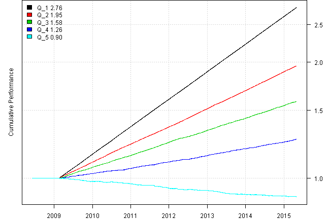
toc(1); Elapsed time is 0.03 seconds
toc(2); Elapsed time is 28.31 seconds
Aside: Rcpp helper function testing:
#*****************************************************************
# Compile Rcpp helper function to compute running window standard deviation in parallel
#*****************************************************************
# [RcppParallel help site](http://rcppcore.github.io/RcppParallel/)
# [RcppParallel source code](https://github.com/RcppCore/RcppParallel)
# [RcppParallel introduction](http://dirk.eddelbuettel.com/blog/2014/07/16/#introducing_rcppparallel)
# [RcppParallel gallery](http://gallery.rcpp.org/articles/parallel-distance-matrix/)
# defaultNumThreads()
#[High performance functions with Rcpp](http://adv-r.had.co.nz/Rcpp.html)
#
# make sure to install [Rtools on windows](http://cran.r-project.org/bin/windows/Rtools/)
load.packages('Rcpp')
load.packages('RcppParallel')
sourceCpp('runsd.cpp')

# test - generate random data
n = 24
nperiods = 10 * 252
ret = matrix(rnorm(n*nperiods), nc=n)

# compute running window standard deviation using Rcpp
cp.sd252 = cp_run_sd(ret, 252)

# compute running window standard deviation using R
library(SIT)
load.packages('quantmod')
r.sd252 = bt.apply.matrix(ret, runSD, 252)

print(test.equality(r.sd252, cp.sd252))| item1 | item2 | equal |
|---|---|---|
| r.sd252 | cp.sd252 | TRUE |
# compare performance
library(rbenchmark)
res <- benchmark(
			cp_run_sd(ret, 252),
			bt.apply.matrix(ret, runSD, 252),
			replications = 20,
			order="relative")
print(res[,1:4])| rownames(x) | test | replications | elapsed | relative |
|---|---|---|---|---|
| 1 | cp_run_sd(ret, 252) | 20 | 0.16 | 1.000 |
| 2 | bt.apply.matrix(ret, runSD, 252) | 20 | 0.94 | 5.875 |
(this report was produced on: 2015-05-01)