Logical Invest Permanent Portfolio
08 Dec 2014To install Systematic Investor Toolbox (SIT) please visit About page.
Look at Vangelis Maderakis’s blog post: Will We Ever Kill The Bug?
The Permanent Portfolio: Stocks, Bonds, Gold, Cash, 25% each
Load historical data for SPY,TLT,GLD,SHY.
#*****************************************************************
# Load historical data
#*****************************************************************
library(SIT)
load.packages('quantmod')
tickers = spl('SPY,TLT,GLD,SHY')

data <- new.env()
getSymbols(tickers, src = 'yahoo', from = '1970-01-01', env = data, auto.assign = T)
extend.data.proxy(data)
for(i in ls(data)) data[[i]] = adjustOHLC(data[[i]], use.Adjusted=T)
bt.prep(data, align='remove.na')
Now we ready to back-test our strategy:
#*****************************************************************
# Code Strategies
#*****************************************************************
prices = data$prices
	n = ncol(prices)
	nperiods = nrow(prices)
period.ends = endpoints(prices, 'years')


models = list()

#*****************************************************************
# Code Strategies, SPY - Buy & Hold
#*****************************************************************
data$weight[] = NA
	data$weight$SPY = 1
models$SPY = bt.run.share(data, clean.signal=T, silent=T)

#*****************************************************************
# Code Strategies, Equal Weight, re-balanced
#*****************************************************************
target.allocation = prices
	target.allocation[] = rep.row(rep(1/n,n), nperiods)

data$weight[] = NA
	data$weight[period.ends,] = target.allocation[period.ends,]
models$permanent.y = bt.run.share(data, clean.signal=F, silent=T)

#*****************************************************************
# Same monthly
#*****************************************************************
period.ends = endpoints(prices, 'months')

weight.equal = target.allocation

data$weight[] = NA
	data$weight[period.ends,] = weight.equal[period.ends,]
models$permanent.m = bt.run.share(data, clean.signal=F, silent=T)

#*****************************************************************
# Volatility Targeting
#*****************************************************************
ret.log = bt.apply.matrix(prices, ROC, type='continuous')
hist.vol = sqrt(252) * bt.apply.matrix(ret.log, runSD, n = 21)
weight.risk = weight.equal / hist.vol
	weight.risk = weight.risk / rowSums(weight.risk)

data$weight[] = NA
	data$weight[period.ends,] = weight.risk[period.ends,]
models$volatility = bt.run.share(data, clean.signal=F, silent=T)

#*****************************************************************
# Volatility Targeting 2
#*****************************************************************
weight.risk = iif(hist.vol > bt.apply.matrix(hist.vol, SMA, 21),
				weight.equal / 2, weight.equal)
weight.risk$SHY = weight.risk$SHY + 1 - rowSums(weight.risk)

data$weight[] = NA
	data$weight[period.ends,] = weight.risk[period.ends,]
models$volatility2 = bt.run.share(data, clean.signal=F, silent=T)

#*****************************************************************
# Momentum
# Lets try by pulling 15% of equity from the worst asset.
# divide the proceeds in three and buy equal amounts
#*****************************************************************
momentum = prices / mlag(prices, 6*21) - 1
	worst.asset = ntop(momentum, 1, F)
	penalty = 1/n * 0.15
weight.momentum = weight.equal - penalty * worst.asset + penalty * (1-worst.asset)/(n-1)

data$weight[] = NA
	data$weight[period.ends,] = weight.momentum[period.ends,]
models$momentum = bt.run.share(data, clean.signal=F, silent=T)


#*****************************************************************
# Mean Reversion
# sell shares of the best short-term performer and distribute the money to the others
#*****************************************************************
mean.reversion = prices / mlag(prices, 1*21) - 1
	best.asset = ntop(mean.reversion, 1)
	penalty = 1/n * 0.15
weight.mean.reversion = weight.equal - penalty * best.asset + penalty * (1-best.asset)/(n-1)

data$weight[] = NA
	data$weight[period.ends,] = weight.mean.reversion[period.ends,]
models$mean.reversion = bt.run.share(data, clean.signal=F, silent=T)

#*****************************************************************
# Timing
# assets price is below its own 200-day simple moving average then we sell it
#*****************************************************************
sma200 = bt.apply.matrix(prices, SMA, 200)
weight.timing = iif(prices > sma200, weight.equal, 0)
weight.timing$SHY = weight.timing$SHY + 1 - rowSums(weight.timing)

data$weight[] = NA
	data$weight[period.ends,] = weight.timing[period.ends,]
models$timing = bt.run.share(data, clean.signal=F, silent=T)


#*****************************************************************
# Create Report
#*****************************************************************
plotbt(models, plotX = T, log = 'y', LeftMargin = 3, main = NULL)
mtext('Cumulative Performance', side = 2, line = 1)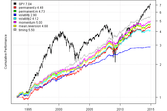
print(plotbt.strategy.sidebyside(models, make.plot=F, return.table=T))| SPY | permanent.y | permanent.m | volatility | volatility2 | momentum | mean.reversion | timing | |
|---|---|---|---|---|---|---|---|---|
| Period | Jan1993 - Dec2014 | Jan1993 - Dec2014 | Jan1993 - Dec2014 | Jan1993 - Dec2014 | Jan1993 - Dec2014 | Jan1993 - Dec2014 | Jan1993 - Dec2014 | Jan1993 - Dec2014 |
| Cagr | 9.33 | 7.09 | 7.36 | 4.98 | 6.68 | 7.64 | 7.31 | 8.1 |
| Sharpe | 0.57 | 1.09 | 1.11 | 1.57 | 1.23 | 1.16 | 1.11 | 1.42 |
| DVR | 0.42 | 1.01 | 1.04 | 1.56 | 1.17 | 1.09 | 1.04 | 1.34 |
| Volatility | 19.09 | 6.57 | 6.67 | 3.17 | 5.47 | 6.6 | 6.64 | 5.69 |
| MaxDD | -55.19 | -14.18 | -15.07 | -5.58 | -10.34 | -14.68 | -14.42 | -7.13 |
| AvgDD | -2.1 | -1 | -0.94 | -0.41 | -0.82 | -0.97 | -0.93 | -0.78 |
| VaR | -1.91 | -0.65 | -0.64 | -0.29 | -0.54 | -0.64 | -0.64 | -0.57 |
| CVaR | -2.84 | -0.93 | -0.92 | -0.44 | -0.77 | -0.92 | -0.92 | -0.81 |
| Exposure | 99.98 | 95.81 | 99.98 | 99.21 | 99.98 | 99.98 | 99.98 | 99.98 |
print(last.trades(models$top1, make.plot=F, return.table=T))#*****************************************************************
# Same for 2014
#*****************************************************************
models1 = bt.trim(models, dates = '2014')
#*****************************************************************
# Create Report
#*****************************************************************
plotbt(models1, plotX = T, log = 'y', LeftMargin = 3, main = NULL)
mtext('Cumulative Performance', side = 2, line = 1)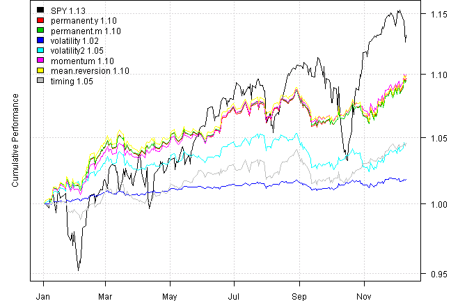
print(plotbt.strategy.sidebyside(models1, make.plot=F, return.table=T))| SPY | permanent.y | permanent.m | volatility | volatility2 | momentum | mean.reversion | timing | |
|---|---|---|---|---|---|---|---|---|
| Period | Jan2014 - Dec2014 | Jan2014 - Dec2014 | Jan2014 - Dec2014 | Jan2014 - Dec2014 | Jan2014 - Dec2014 | Jan2014 - Dec2014 | Jan2014 - Dec2014 | Jan2014 - Dec2014 |
| Cagr | 14.09 | 10.3 | 10.17 | 1.91 | 4.88 | 10.61 | 10.54 | 4.87 |
| Sharpe | 1.17 | 2.12 | 2.09 | 1.45 | 1.34 | 2.27 | 2.13 | 1.25 |
| DVR | 0.97 | 1.67 | 1.63 | 1.12 | 0.45 | 1.91 | 1.63 | 0.9 |
| Volatility | 10.83 | 4.77 | 4.77 | 1.33 | 3.71 | 4.57 | 4.89 | 3.64 |
| MaxDD | -7.27 | -2.65 | -2.57 | -0.76 | -2.79 | -2.44 | -2.49 | -2.57 |
| AvgDD | -1.35 | -0.59 | -0.6 | -0.16 | -0.54 | -0.56 | -0.61 | -0.61 |
| VaR | -1.15 | -0.46 | -0.47 | -0.13 | -0.37 | -0.46 | -0.48 | -0.37 |
| CVaR | -1.73 | -0.65 | -0.64 | -0.19 | -0.54 | -0.63 | -0.64 | -0.59 |
| Exposure | 100 | 100 | 100 | 100 | 100 | 100 | 100 | 100 |
#*****************************************************************
# Same for last 5 years
#*****************************************************************
models1 = bt.trim(models, dates = '2010::')


#*****************************************************************
# Create Report
#*****************************************************************
plotbt(models1, plotX = T, log = 'y', LeftMargin = 3, main = NULL)
mtext('Cumulative Performance', side = 2, line = 1)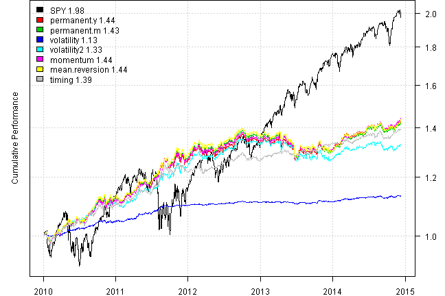
print(plotbt.strategy.sidebyside(models1, make.plot=F, return.table=T))| SPY | permanent.y | permanent.m | volatility | volatility2 | momentum | mean.reversion | timing | |
|---|---|---|---|---|---|---|---|---|
| Period | Jan2010 - Dec2014 | Jan2010 - Dec2014 | Jan2010 - Dec2014 | Jan2010 - Dec2014 | Jan2010 - Dec2014 | Jan2010 - Dec2014 | Jan2010 - Dec2014 | Jan2010 - Dec2014 |
| Cagr | 14.88 | 7.64 | 7.48 | 2.55 | 5.96 | 7.68 | 7.59 | 6.96 |
| Sharpe | 0.97 | 1.23 | 1.21 | 1.73 | 1.15 | 1.26 | 1.23 | 1.34 |
| DVR | 0.9 | 1.05 | 0.98 | 1.44 | 0.88 | 1.05 | 0.98 | 1.26 |
| Volatility | 15.86 | 6.3 | 6.31 | 1.51 | 5.27 | 6.22 | 6.29 | 5.28 |
| MaxDD | -18.61 | -8.05 | -8.85 | -1.1 | -6.74 | -7.91 | -8.96 | -3.7 |
| AvgDD | -1.68 | -0.96 | -0.95 | -0.18 | -0.79 | -0.95 | -0.91 | -0.71 |
| VaR | -1.61 | -0.62 | -0.63 | -0.15 | -0.51 | -0.63 | -0.62 | -0.54 |
| CVaR | -2.42 | -0.92 | -0.92 | -0.21 | -0.81 | -0.91 | -0.92 | -0.8 |
| Exposure | 100 | 100 | 100 | 100 | 100 | 100 | 100 | 100 |
Finally let’s include some ‘newer’ asset classes that were not easily accessible during the 80’s. Convertible bonds (CWB) Foreign bonds (PCY) Inflation protected Treasuries (TIP)
A few notes about R code and how it works.
For example, below I want to create an xts object with target allocation.
target.allocation = prices
	target.allocation[] = rep.row(rep(1/n,n), nperiods)
The trick is to take an existing xts object, in this example prices, and
override it’s content with target values. The [] operator in front of target.allocation
indicates that we are only changing content of target.allocation, but keeping all other
attributes.
Another example is pulling 15% of equity from the worst asset, and divide the proceeds in three and buy equal amounts
	worst.asset = ntop(momentum, 1, F)
	penalty = 1/n * 0.15
	weight.momentum = weight.equal - penalty * worst.asset + penalty * (1-worst.asset)/(n-1)
First we find worst.asset, i.e. it will contain 1’s in the location of the worst asset and
0’s everywhere else:
print(tail(worst.asset,10))| GLD | SHY | SPY | TLT | |
|---|---|---|---|---|
| 2014-11-28 | 1 | 0 | 0 | 0 |
| 2014-12-01 | 1 | 0 | 0 | 0 |
| 2014-12-02 | 1 | 0 | 0 | 0 |
| 2014-12-03 | 1 | 0 | 0 | 0 |
| 2014-12-04 | 1 | 0 | 0 | 0 |
| 2014-12-05 | 1 | 0 | 0 | 0 |
| 2014-12-08 | 1 | 0 | 0 | 0 |
| 2014-12-09 | 1 | 0 | 0 | 0 |
| 2014-12-10 | 1 | 0 | 0 | 0 |
| 2014-12-11 | 1 | 0 | 0 | 0 |
Next, we know that in our target allocation each asset get’s 1/n weight, so the
worst asset will get a penalty equal to 15% of it’s weight. I.e.
print(tail(weight.equal,10))| GLD | SHY | SPY | TLT | |
|---|---|---|---|---|
| 2014-11-28 | 0.25 | 0.25 | 0.25 | 0.25 |
| 2014-12-01 | 0.25 | 0.25 | 0.25 | 0.25 |
| 2014-12-02 | 0.25 | 0.25 | 0.25 | 0.25 |
| 2014-12-03 | 0.25 | 0.25 | 0.25 | 0.25 |
| 2014-12-04 | 0.25 | 0.25 | 0.25 | 0.25 |
| 2014-12-05 | 0.25 | 0.25 | 0.25 | 0.25 |
| 2014-12-08 | 0.25 | 0.25 | 0.25 | 0.25 |
| 2014-12-09 | 0.25 | 0.25 | 0.25 | 0.25 |
| 2014-12-10 | 0.25 | 0.25 | 0.25 | 0.25 |
| 2014-12-11 | 0.25 | 0.25 | 0.25 | 0.25 |
	weight.momentum = weight.equal - penalty * worst.asset
print(tail(weight.momentum,10))| GLD | SHY | SPY | TLT | |
|---|---|---|---|---|
| 2014-11-28 | 0.2125 | 0.25 | 0.25 | 0.25 |
| 2014-12-01 | 0.2125 | 0.25 | 0.25 | 0.25 |
| 2014-12-02 | 0.2125 | 0.25 | 0.25 | 0.25 |
| 2014-12-03 | 0.2125 | 0.25 | 0.25 | 0.25 |
| 2014-12-04 | 0.2125 | 0.25 | 0.25 | 0.25 |
| 2014-12-05 | 0.2125 | 0.25 | 0.25 | 0.25 |
| 2014-12-08 | 0.2125 | 0.25 | 0.25 | 0.25 |
| 2014-12-09 | 0.2125 | 0.25 | 0.25 | 0.25 |
| 2014-12-10 | 0.2125 | 0.25 | 0.25 | 0.25 |
| 2014-12-11 | 0.2125 | 0.25 | 0.25 | 0.25 |
Please notice that we still need to distribute the weight which is taken away from the worst asset.
1-worst.asset is matrix that has 0’s for the worst asset and 1’s every there else.
print(tail(1-worst.asset,10))| GLD | SHY | SPY | TLT | |
|---|---|---|---|---|
| 2014-11-28 | 0 | 1 | 1 | 1 |
| 2014-12-01 | 0 | 1 | 1 | 1 |
| 2014-12-02 | 0 | 1 | 1 | 1 |
| 2014-12-03 | 0 | 1 | 1 | 1 |
| 2014-12-04 | 0 | 1 | 1 | 1 |
| 2014-12-05 | 0 | 1 | 1 | 1 |
| 2014-12-08 | 0 | 1 | 1 | 1 |
| 2014-12-09 | 0 | 1 | 1 | 1 |
| 2014-12-10 | 0 | 1 | 1 | 1 |
| 2014-12-11 | 0 | 1 | 1 | 1 |
So penalty * (1-worst.asset)/(n-1) distributes the penalty weight equally among the rest of
assets. I.e. `n-1’ assets. And now the final portfolio weight is sums up to one.
	weight.momentum = weight.equal - penalty * worst.asset + penalty * (1-worst.asset)/(n-1)
print(tail(weight.momentum,10))| GLD | SHY | SPY | TLT | |
|---|---|---|---|---|
| 2014-11-28 | 0.2125 | 0.2625 | 0.2625 | 0.2625 |
| 2014-12-01 | 0.2125 | 0.2625 | 0.2625 | 0.2625 |
| 2014-12-02 | 0.2125 | 0.2625 | 0.2625 | 0.2625 |
| 2014-12-03 | 0.2125 | 0.2625 | 0.2625 | 0.2625 |
| 2014-12-04 | 0.2125 | 0.2625 | 0.2625 | 0.2625 |
| 2014-12-05 | 0.2125 | 0.2625 | 0.2625 | 0.2625 |
| 2014-12-08 | 0.2125 | 0.2625 | 0.2625 | 0.2625 |
| 2014-12-09 | 0.2125 | 0.2625 | 0.2625 | 0.2625 |
| 2014-12-10 | 0.2125 | 0.2625 | 0.2625 | 0.2625 |
| 2014-12-11 | 0.2125 | 0.2625 | 0.2625 | 0.2625 |
(this report was produced on: 2014-12-12)