Loading Historical Stock Data
13 Nov 2014To install Systematic Investor Toolbox (SIT) please visit About page.
Historical Stock Data is critical for testing your investment strategies. There are many ways to load Historical Stock Data in to your R session. Below I show 4 different approaches to load historical stock data:
- Download Historical Stock quotes from Yahoo Fiance with getSymbols function from quantmod package
- Load Historical Stock data from the csv files you saved from Yahoo Fiance
- Load Historical Stock data from your custom files
- Load Historical Stock from one csv file, where each column represents one stock
In the code below I demonstrate these 4 methods and use loaded data to run a back-test:
Loading Historical Prices:
	#*****************************************************************
	# Load historical data
	#******************************************************************
	library(SIT)
	load.packages('quantmod')

	stock.folder = 'c:\\Stocks\\Data\\'
	tickers = spl('UUP,EMB,HYG')

	data <- new.env()

	# load historical data, select data load method
	data.load.method = 'basic'

	if(data.load.method == 'basic') {
        # quantmod - getSymbols
        getSymbols(tickers, src = 'yahoo', from = '1970-01-01', env = data, auto.assign = T)
	}else if(data.load.method == 'basic.local') {
        # if you saved yahoo historical price files localy
        getSymbols.sit(tickers, src = 'yahoo', from = '1980-01-01', env = data, auto.assign = T, stock.folder = stock.folder)
	}else if(data.load.method == 'custom.local') {
        # custom format historical price files
        for(n in tickers) {
            data[[n]] = read.xts(paste(stock.folder, n, '.csv', sep=''), format='%m/%d/%Y')
        }
	}else if(data.load.method == 'custom.one.file') {
        # read from one csv file, column headers are tickers
        filename = 'hex.csv'
        all.data = read.xts(paste(stock.folder, filename, sep=''), format='%m/%d/%Y')
        for(n in names(all.data)) {
            data[[n]] = all.data[,n]
            colnames(data[[n]]) = 'Close'
            data[[n]]$Adjusted = data[[n]]$Open = data[[n]]$High = data[[n]]$Low = data[[n]]$Close
        }
	}

	# prepare data for back test
		for(i in ls(data)) data[[i]] = adjustOHLC(data[[i]], use.Adjusted=T)
	bt.prep(data, align='remove.na')


	#*****************************************************************
	# Code Strategies
	#******************************************************************
	prices = data$prices
	n = ncol(prices)

	models = list()

	# find period ends
	period.ends = endpoints(prices, 'months')
		period.ends = period.ends[period.ends > 0]

	obj = portfolio.allocation.helper(data$prices, period.ends=period.ends, lookback.len = 250,
		min.risk.fns = list(EW=equal.weight.portfolio,
                        RP=risk.parity.portfolio(),
                        MV=min.var.portfolio,
                        MC=min.corr.portfolio)
	)
20 , percent = 9.7% 30 , percent = 23.6% 40 , percent = 37.5% 50 , percent = 51.4% 60 , percent = 65.3% 70 , percent = 79.2% 80 , percent = 93.1%
models = create.strategies(obj, data)$modelsEW , percent = 25% Latest weights :
| EMB | HYG | UUP | |
|---|---|---|---|
| 2014-12-05 | 296.3226 | 369.099 | 1405.877 |
Performance summary : CAGR Best Worst 5.4 2.2 -3.1
RP , percent = 50% Latest weights :
| EMB | HYG | UUP | |
|---|---|---|---|
| 2014-12-05 | 294.9029 | 402.3187 | 1286.081 |
Performance summary : CAGR Best Worst 4.4 1.8 -2.7
MV , percent = 75% Latest weights :
| EMB | HYG | UUP | |
|---|---|---|---|
| 2014-12-05 | 291.1793 | 336.6892 | 1553.726 |
Performance summary : CAGR Best Worst 3 1.7 -2.1
MC , percent = 100% Latest weights :
| EMB | HYG | UUP | |
|---|---|---|---|
| 2014-12-05 | 200.0815 | 200.7362 | 2503.768 |
Performance summary : CAGR Best Worst 2 1.8 -2
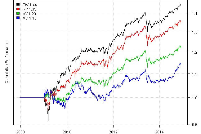
Finally let’s make a report:
	#*****************************************************************
	# Create Report
	#******************************************************************
	plotbt(models, plotX = T, log = 'y', LeftMargin = 3, main = NULL)
		mtext('Cumulative Performance', side = 2, line = 1)
print(plotbt.strategy.sidebyside(models, make.plot=F, return.table=T))| EW | RP | MV | MC | |
|---|---|---|---|---|
| Period | Dec2007 - Dec2014 | Dec2007 - Dec2014 | Dec2007 - Dec2014 | Dec2007 - Dec2014 |
| Cagr | 5.41 | 4.45 | 2.97 | 2.02 |
| Sharpe | 1.11 | 0.97 | 0.67 | 0.43 |
| DVR | 1.05 | 0.92 | 0.61 | 0.31 |
| Volatility | 4.87 | 4.59 | 4.56 | 4.95 |
| MaxDD | -11.05 | -7.78 | -6.59 | -8.15 |
| AvgDD | -0.81 | -0.82 | -0.91 | -1.36 |
| VaR | -0.41 | -0.41 | -0.41 | -0.48 |
| CVaR | -0.74 | -0.72 | -0.71 | -0.74 |
| Exposure | 85.12 | 85.12 | 85.12 | 85.12 |
(this report was produced on: 2014-12-07)