Timing in High Yield Bonds
10 Nov 2014To install Systematic Investor Toolbox (SIT) please visit About page.
A quick test of the results presented at Predicting Bonds with Stocks: A Strategy to Improve Timing in Corporate and High Yield Bonds.
First, let’s load Load Systematic Investor Toolbox (SIT):
Load Historical Prices from Yahoo Finance:
  #*****************************************************************
  # Load historical data
  #******************************************************************
  library(SIT)
  load.packages('quantmod')
  tickers = spl('SPY,HYG+VWEHX,LQD+VWESX,SHY+VFISX')

  data <- new.env()
	getSymbols.extra(tickers, src = 'yahoo', from = '1980-01-01', env = data, set.symbolnames = F, auto.assign = T)
		#bt.start.dates(data)
    for(i in ls(data)) data[[i]] = adjustOHLC(data[[i]], use.Adjusted=T)
  bt.prep(data, align='remove.na')
Look at correlations:
  #*****************************************************************
  # Look at Correlations
  #******************************************************************

  prices = data$prices

  plota.matplot(scale.one(prices))
vis.cor(prices, 'days')Daily Correlations:
| HYG | LQD | SHY | |
|---|---|---|---|
| LQD | 37 | ||
| SHY | -1 | 46 | |
| SPY | 45 | 5 | -21 |
vis.cor(prices, 'weeks')Weekly Correlations:
| HYG | LQD | SHY | |
|---|---|---|---|
| LQD | 43 | ||
| SHY | -1 | 59 | |
| SPY | 56 | 9 | -16 |
vis.cor(prices, 'bi-weeks')Bi-Weekly Correlations:
| HYG | LQD | SHY | |
|---|---|---|---|
| LQD | 45 | ||
| SHY | -7 | 53 | |
| SPY | 57 | 11 | -20 |
vis.cor(prices, 'months')Monthly Correlations:
| HYG | LQD | SHY | |
|---|---|---|---|
| LQD | 59 | ||
| SHY | -10 | 46 | |
| SPY | 61 | 20 | -23 |
SPY has high correlated with HYG, but correlation with LQD is not very high.
Look at strategies that go long if the close is above the SMA and otherwise, below SMA, allocate to cash, represented by SHY:
  #*****************************************************************
  # Code Strategies
  #******************************************************************
  prices = data$prices
  n = len(tickers)

  sma.20 = bt.apply.matrix(prices, SMA, 20)
  signal = prices > sma.20

  models = list()

  #*****************************************************************
  # Code Strategies
  #******************************************************************
  data$weight[] = NA
    data$weight$HYG = signal$HYG
    data$weight$SHY = !signal$HYG
  models$HYG.HYG.20 = bt.run.share(data, silent=T, clean.signal=T)

  data$weight[] = NA
    data$weight$HYG = signal$SPY
    data$weight$SHY = !signal$SPY
  models$HYG.SPY.20 = bt.run.share(data, silent=T, clean.signal=T)

  data$weight[] = NA
    data$weight$LQD = signal$LQD
    data$weight$SHY = !signal$LQD
  models$LQD.LQD.20 = bt.run.share(data, silent=T, clean.signal=T)

  data$weight[] = NA
    data$weight$LQD = signal$SPY
    data$weight$SHY = !signal$SPY
  models$LQD.SPY.20 = bt.run.share(data, silent=T, clean.signal=T)
Create Report:
  #*****************************************************************
  # Create Report
  #******************************************************************
  #strategy.performance.snapshoot(models, T)
  plotbt(models, plotX = T, log = 'y', LeftMargin = 3, main = NULL)
    mtext('Cumulative Performance', side = 2, line = 1)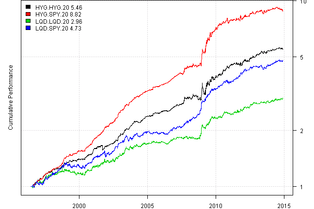
print(plotbt.strategy.sidebyside(models, make.plot=F, return.table=T))| HYG.HYG.20 | HYG.SPY.20 | LQD.LQD.20 | LQD.SPY.20 | |
|---|---|---|---|---|
| Period | Jun1996 - Dec2014 | Jun1996 - Dec2014 | Jun1996 - Dec2014 | Jun1996 - Dec2014 |
| Cagr | 9.63 | 12.51 | 6.04 | 8.77 |
| Sharpe | 1.6 | 2.1 | 1.09 | 1.56 |
| DVR | 1.51 | 1.96 | 1.03 | 1.41 |
| Volatility | 5.86 | 5.69 | 5.54 | 5.5 |
| MaxDD | -13.45 | -6.37 | -8.84 | -7.49 |
| AvgDD | -0.85 | -0.59 | -1.1 | -0.71 |
| VaR | -0.37 | -0.37 | -0.54 | -0.53 |
| CVaR | -0.78 | -0.71 | -0.8 | -0.77 |
| Exposure | 99.57 | 99.57 | 99.57 | 99.57 |
Please note that using SPY as a timing proxy improves results for both HYG and LQD.
Previously, I have already observed that SPY has better trimming power than security’s own moving average. For example, below let’s look at trading Sector SPDRs with timing based on their own moving average vs timing based SPY’s moving average.
  #*****************************************************************
  # Load historical data
  #******************************************************************
	load.packages('quantmod')
	tickers = spl('SPY,XLY,XLP,XLE,XLF,XLV,XLI,XLB,XLK,XLU,SHY+VFISX')

	data <- new.env()
	getSymbols.extra(tickers, src = 'yahoo', from = '1980-01-01', env = data, set.symbolnames = F, auto.assign = T)
		for(i in ls(data)) data[[i]] = adjustOHLC(data[[i]], use.Adjusted=T)
	bt.prep(data, align='remove.na')

  #*****************************************************************
  # Look at Correlations
  #******************************************************************
  prices = data$prices

  plota.matplot(scale.one(prices))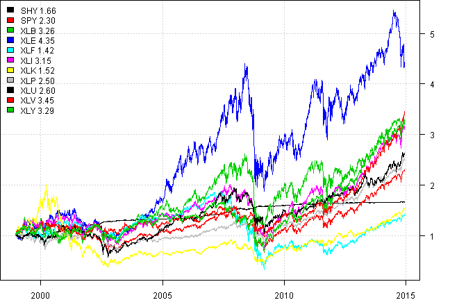
vis.cor(prices, 'months')Monthly Correlations:
| SHY | SPY | XLB | XLE | XLF | XLI | XLK | XLP | XLU | XLV | |
|---|---|---|---|---|---|---|---|---|---|---|
| SPY | -32 | |||||||||
| XLB | -26 | 80 | ||||||||
| XLE | -23 | 62 | 65 | |||||||
| XLF | -18 | 82 | 69 | 46 | ||||||
| XLI | -28 | 89 | 85 | 62 | 79 | |||||
| XLK | -34 | 84 | 55 | 39 | 50 | 64 | ||||
| XLP | -14 | 59 | 46 | 38 | 57 | 54 | 27 | |||
| XLU | -17 | 47 | 42 | 48 | 40 | 46 | 20 | 54 | ||
| XLV | -23 | 79 | 61 | 40 | 64 | 69 | 62 | 52 | 44 | |
| XLY | -25 | 86 | 75 | 44 | 77 | 82 | 68 | 50 | 35 | 69 |
  #*****************************************************************
  # Code Strategies
  #******************************************************************
  prices = data$prices
  n = len(tickers)

  sma.20 = bt.apply.matrix(prices, SMA, 20)
  signal = prices > sma.20

  models = list()

  #*****************************************************************
  # Code Strategies
  #******************************************************************
  for(ticker in spl('XLY,XLP,XLE,XLF,XLV,XLI,XLB,XLK,XLU')) {
    data$weight[] = NA
      data$weight[,ticker] = signal[,ticker]
      data$weight$SHY = !signal[,ticker]
    models[[paste(ticker,ticker,'20',sep='.')]] = bt.run.share(data, silent=T, clean.signal=T)

    data$weight[] = NA
      data$weight[,ticker] = signal$SPY
      data$weight$SHY = !signal$SPY
    models[[paste(ticker,'SPY','20',sep='.')]] = bt.run.share(data, silent=T, clean.signal=T)
  }

  #*****************************************************************
  # Create Report
  #******************************************************************
  #strategy.performance.snapshoot(models, T)
  plotbt(models, plotX = T, log = 'y', LeftMargin = 3, main = NULL)
    mtext('Cumulative Performance', side = 2, line = 1)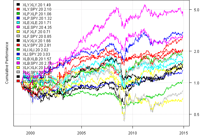
print(plotbt.strategy.sidebyside(models, make.plot=F, return.table=T))| XLY.XLY.20 | XLY.SPY.20 | XLP.XLP.20 | XLP.SPY.20 | XLE.XLE.20 | XLE.SPY.20 | XLF.XLF.20 | XLF.SPY.20 | XLV.XLV.20 | XLV.SPY.20 | XLI.XLI.20 | XLI.SPY.20 | XLB.XLB.20 | XLB.SPY.20 | XLK.XLK.20 | XLK.SPY.20 | XLU.XLU.20 | XLU.SPY.20 | |
|---|---|---|---|---|---|---|---|---|---|---|---|---|---|---|---|---|---|---|
| Period | Dec1998 - Dec2014 | Dec1998 - Dec2014 | Dec1998 - Dec2014 | Dec1998 - Dec2014 | Dec1998 - Dec2014 | Dec1998 - Dec2014 | Dec1998 - Dec2014 | Dec1998 - Dec2014 | Dec1998 - Dec2014 | Dec1998 - Dec2014 | Dec1998 - Dec2014 | Dec1998 - Dec2014 | Dec1998 - Dec2014 | Dec1998 - Dec2014 | Dec1998 - Dec2014 | Dec1998 - Dec2014 | Dec1998 - Dec2014 | Dec1998 - Dec2014 |
| Cagr | 2.51 | 4.75 | 0.35 | 1.74 | 3.41 | 9.65 | -2.08 | -1.03 | 3.21 | 6.69 | 4.49 | 7.19 | 2.85 | 6.64 | 2.67 | 4.73 | 2.11 | 4.6 |
| Sharpe | 0.24 | 0.38 | 0.09 | 0.22 | 0.28 | 0.6 | 0.01 | 0.06 | 0.33 | 0.62 | 0.38 | 0.56 | 0.25 | 0.47 | 0.24 | 0.36 | 0.23 | 0.44 |
| DVR | 0.11 | 0.32 | 0 | 0.17 | 0.12 | 0.53 | 0 | 0.01 | 0.23 | 0.51 | 0.32 | 0.51 | 0.12 | 0.37 | 0.16 | 0.3 | 0.06 | 0.34 |
| Volatility | 15.25 | 15.06 | 10.4 | 10.15 | 17.9 | 18.08 | 21.77 | 22.14 | 11.56 | 11.54 | 14.26 | 14.09 | 16.48 | 16.75 | 16.47 | 16.91 | 12.2 | 11.94 |
| MaxDD | -41.57 | -37.15 | -43.46 | -37.35 | -51.66 | -37.93 | -68.29 | -69.6 | -37.21 | -18.67 | -34.49 | -33.73 | -50 | -33.21 | -41.73 | -39.8 | -41.02 | -32.18 |
| AvgDD | -3.47 | -3.72 | -6.51 | -2.44 | -6.02 | -3.41 | -6.57 | -5.01 | -2.28 | -2.52 | -2.8 | -3.04 | -4.19 | -3.57 | -3.76 | -3.03 | -2.82 | -2.54 |
| VaR | -1.52 | -1.52 | -1.03 | -1 | -1.87 | -1.81 | -1.65 | -1.74 | -1.19 | -1.11 | -1.34 | -1.34 | -1.72 | -1.7 | -1.72 | -1.72 | -1.34 | -1.24 |
| CVaR | -2.43 | -2.36 | -1.66 | -1.61 | -2.88 | -2.85 | -3.18 | -3.2 | -1.86 | -1.75 | -2.29 | -2.22 | -2.6 | -2.61 | -2.75 | -2.77 | -1.97 | -1.88 |
| Exposure | 99.5 | 99.5 | 99.5 | 99.5 | 99.5 | 99.5 | 99.5 | 99.5 | 99.5 | 99.5 | 99.5 | 99.5 | 99.5 | 99.5 | 99.5 | 99.5 | 99.5 | 99.5 |
In all cases, timing signal based on SPY improved strategy returns. Please use left(←) and right(→) arrow keys to scroll this wide table.
(this report was produced on: 2014-12-07)