Financial Turbulence Example
01 Dec 2012To install Systematic Investor Toolbox (SIT) please visit About page.
Today, I want to highlight the Financial Turbulence Index idea introduced by Mark Kritzman and Yuanzhen Li in the Skulls, Financial Turbulence, and Risk Management paper. Timely Portfolio did a great series of posts about Financial Turbulence:
As example, I will compute Financial Turbulence for the equal weight index of G10 Currencies.
I created a helper function get.G10() function in data.r at github to download historical data for G10 Currencies from FRED.
Let’s compute Financial Turbulence Index for G10 Currencies.
	#*****************************************************************
	# Load historical data
	#*****************************************************************
	library(SIT)
	load.packages('quantmod')

	fx = get.G10()
		nperiods = nrow(fx)

	# Check data, plot FX vols
	ret = diff(log(fx))
	hist.vol = sqrt(252) * bt.apply.matrix(ret, runSD, n = 20)
	plota.matplot(hist.vol,main='FX Vol')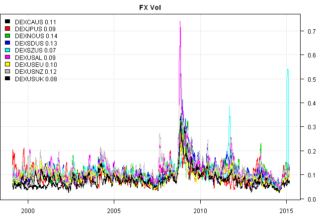
Swiss currency, DEXSZUS - Switzerland/U.S., dropeed 13% in a single day due to removal of trading restrictions.
	#*****************************************************************
	# Rolling estimate of the Financial Turbulence for G10 Currencies
	#******************************************************************
	turbulence = fx[,1] * NA
		colnames(turbulence) = 'turbulence'
	ret = coredata(fx / mlag(fx) - 1)

	look.back = 252

	for( i in (look.back+1) : nperiods ) {
		temp = ret[(i - look.back + 1):(i-1), ]

		# measures turbulence for the current observation
		turbulence[i] = mahalanobis(ret[i,], colMeans(temp), cov(temp))
	}

	# DEXSZUS - Switzerland/U.S.
print(to.nice(cbind(fx,turbulence)['2015-01-14::2015-01-16',]))| DEXCAUS | DEXJPUS | DEXNOUS | DEXSDUS | DEXSZUS | DEXUSAL | DEXUSEU | DEXUSNZ | DEXUSUK | turbulence | |
|---|---|---|---|---|---|---|---|---|---|---|
| 2015-01-14 | 1.20 | 116.78 | 7.64 | 8.05 | 1.02 | 1.23 | 0.85 | 1.29 | 0.66 | 23.03 |
| 2015-01-15 | 1.19 | 116.95 | 7.65 | 8.14 | 0.89 | 1.22 | 0.86 | 1.28 | 0.66 | 17,225.61 |
| 2015-01-16 | 1.20 | 117.45 | 7.60 | 8.14 | 0.85 | 1.22 | 0.87 | 1.29 | 0.66 | 47.83 |
	#*****************************************************************
	# Plot 30 day average of the Financial Turbulence for G10 Currencies
	#******************************************************************
	plota(EMA( turbulence, 30), type='l',
		main='30 day average of the Financial Turbulence for G10 Currencies')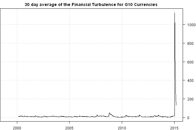
	#*****************************************************************
	# Same plot with 2015-01-15 removed
	#******************************************************************
	turbulence['2015-01-15']=NA
	plota(EMA( ifna.prev(turbulence), 30), type='l',
main='30 day average of the Financial Turbulence for G10 Currencies, 2015-01-15 removed') 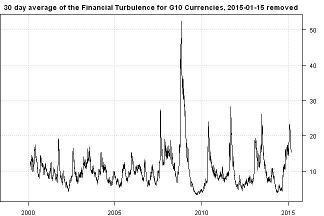
There is a big spike in the index during 2008-2009 period. If you had monitored the Financial Turbulence Index and reduced or hedged your positions during these times, you would be able to reduce your draw-downs and sleep better at night.
To view the complete source code for this example, please have a look at the bt.financial.turbulence.test() function in bt.test.r at github.
(this report was produced on: 2015-03-14)