Filtering Stocks
26 Mar 2015To install Systematic Investor Toolbox (SIT) please visit About page.
I found following discussions interesting and easy to test:
-
NASDAQ 100 Couples by Ripples The similarity measure is based on distance function from TSdist package
Below I will try to adapt a code from the posts:
#*****************************************************************
# Load historical end of day data
#*****************************************************************
library(SIT)
load.packages('quantmod')

tickers = nasdaq.100.components()
	tickers = c('SPY', tickers)

data <- new.env()
getSymbols.extra(tickers, src = 'yahoo', from = '1970-01-01', env = data, set.symbolnames = T, auto.assign = T)
for(i in data$symbolnames) data[[i]] = adjustOHLC(data[[i]], use.Adjusted=T)
#print(bt.start.dates(data))

bt.prep(data, align='keep.all', dates='2000::', fill.gaps=T)

# remove ones with little history
bt.prep.remove.symbols.min.history(data, 5*252)

# show the ones removed
print(setdiff(tickers,names(data$prices)))
FB GOOG KRFT LVNTA LMCA LMCK NXPI TSLA TRIP
#*****************************************************************
# Compute Distance
#*****************************************************************
tickers = names(data$prices)
prices = data$prices
	n = ncol(prices)
	prices = last(prices, 5*252)
	prices = coredata(prices)

load.packages('TSdist')

# all possible combinations
choices = expand.grid(t1=1:n,t2=1:n,KEEP.OUT.ATTRS=F)
	choices = choices[choices$t1 <  choices$t2,]
	n.choices = nrow(choices)
choices = as.matrix(choices)

#*****************************************************************
# Compute over all combinations
#*****************************************************************
# Following is SLOW, let's use all cores
#result = rep(NA, n.choices)
#for(i in 1:n.choices) {
#	result[i] = tsDistances(prices[,choices[i,1]], prices[,choices[i,2]], distance="crosscorrelation")
#	if( i %% 100 == 0) cat(i, '\n')
#}

# Run Cluster
load.packages('parallel')

cl = setup.cluster({library(TSdist)}, 'prices,choices',envir=environment())
out = clusterApplyLB(cl, 1:n.choices, function(i) { tsDistances(prices[,choices[i,1]], prices[,choices[i,2]], distance="crosscorrelation") } )
stopCluster(cl)

result = do.call(c, out)

#*****************************************************************
# Plot
#*****************************************************************
side.by.side.plot = function(index, main=NULL) {
	i = choices[index,1]
	j = choices[index,2]

	plota(prices[,i], type = 'l', LeftMargin=3, col='blue', main=main)
	plota2Y(prices[,j], type='l', las=1, col='red', col.axis = 'red')
	plota.legend(paste(tickers[i], '(rhs),', tickers[j], '(lhs)'), 'blue,red', list(prices[,i],prices[,j]))
}

prices = last(data$prices, 5*252)
index = sort.list(result)

i = index[1]
side.by.side.plot(i, paste('Smallest Dist', result[i]))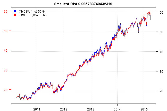
i = last(index)
side.by.side.plot(i, paste('Largest Dist', result[i]))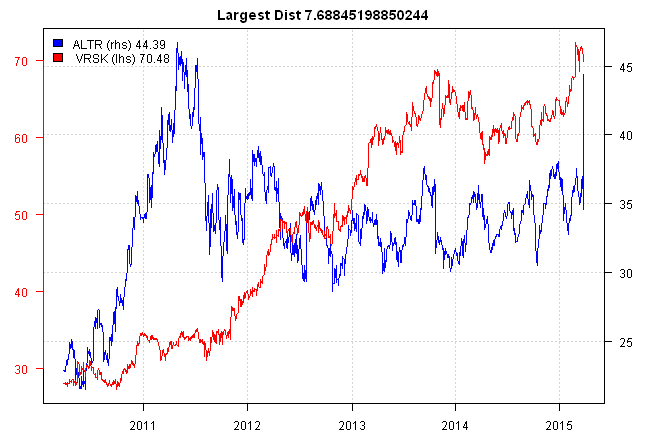
i = index[100]
side.by.side.plot(i, paste('Smallest[100] Dist', result[i]))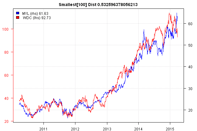
i = last(index,100)[1]
side.by.side.plot(i, paste('Largest[100] Dist', result[i])) 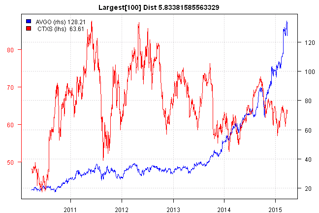
Next let’s look at the second idea: Stocks with upside potential by Eran Raviv
#*****************************************************************
# Compute Qunatile Regressions
#*****************************************************************
prices = data$prices
	n = ncol(prices)
	rets = prices / mlag(prices) - 1
	rets = last(rets, 1 * 252)
	rets = coredata(rets)

load.packages('quantreg')

# Ask the slopes for 20% and 80%
tau = c(.2,.8)

result = matrix(1, nr=n, nc=2)
for(i in 2:n) {
	result[i,1] = rq(rets[,i] ~ rets[,1], tau = tau[1])$coef[2]
	result[i,2] = rq(rets[,i] ~ rets[,1], tau = tau[2])$coef[2]
	if( i %% 100 == 0) cat(i, '\n')
}

ratio = result[,2] / result[,1]

#*****************************************************************
# Plot
#*****************************************************************
rq.plot = function(i, main='') {
	plot(rets[,1], rets[,i], xlab='Market return', ylab='Return', main=paste(tickers[i],main))
		abline(reg = rq(rets[,i] ~ rets[,1], tau = tau[1]), col='red', lwd=2)
		abline(reg = rq(rets[,i] ~ rets[,1], tau = tau[2]), col='red', lwd=2)
		abline(reg = rq(rets[,i] ~ rets[,1], tau = 0.5), col='blue', lwd=2)
}


index = sort.list(ratio)

i = index[1]
rq.plot(i, 'Smallest Dist')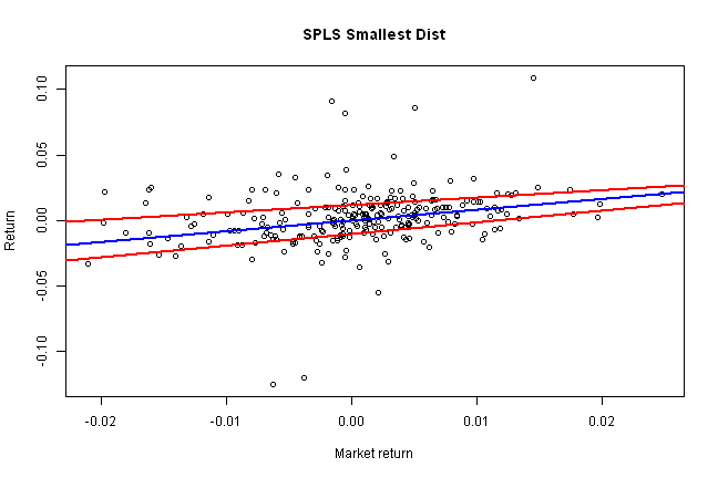
i = last(index)
rq.plot(i,'Largest Dist')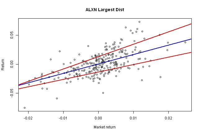
i = index[10]
rq.plot(i,'Smallest[10] Dist')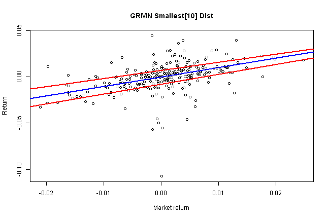
i = last(index,10)[1]
rq.plot(i,'Largest[10] Dist')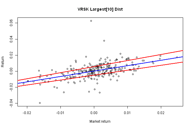
Both concepts work, and show lot’s of promise.
To be continued…
(this report was produced on: 2015-03-29)