Data Proxy - extending time series with proxies
14 Nov 2014To install Systematic Investor Toolbox (SIT) please visit About page.
This page will hold collection of Proxies I collected to extend historical time series.
Note: there are more examples at Composing Synthetic Prices For Extended Historical ETF Data
Commodities:
    #*****************************************************************
    # Load external data
    #******************************************************************
    library(SIT)
    load.packages('quantmod')

raw.data <- new.env()

    # TRJ_CRB file was downloaded from the
    # http://www.corecommodityllc.com/CoreIndexes.aspx
    # select TR/CC-CRB Index-Total Return and click "See Chart"
    # on Chart page click "Download to Spreadsheet" link
    # copy TR_CC-CRB, downloaded file, to data folder
    temp = extract.table.from.webpage( join(readLines("data/TR_CC-CRB")), 'EODValue' )
    temp = join( apply(temp, 1, join, ','), '\n' )
    raw.data$CRB = make.stock.xts( read.xts(temp, format='%m/%d/%y' ) )

    # prfmdata.csv file was downloaded from the http://www.crbequityindexes.com/indexdata-form.php
    # for "TR/J CRB Global Commodity Equity Index", "Total Return", "All Dates"
    raw.data$CRB_2 = make.stock.xts( read.xts('data/prfmdata.csv', format='%m/%d/%Y' ) )

    #*****************************************************************
    # Load historical data
    #******************************************************************
    load.packages('quantmod')

    tickers = spl('GSG,DBC')
    data = new.env()

    data$CRB = raw.data$CRB
    data$CRB_2 = raw.data$CRB_2

    getSymbols(tickers, src = 'yahoo', from = '1970-01-01', env = data, auto.assign = T)
        for(i in ls(data)) data[[i]] = adjustOHLC(data[[i]], use.Adjusted=T)
Look at historical start date for each series:
print(bt.start.dates(data))| Start | |
|---|---|
| CRB | 1994-01-03 |
| CRB_2 | 1999-12-31 |
| DBC | 2006-02-06 |
| GSG | 2006-07-21 |
There are 2 sources of historical commodity index data. Let’s compare them with commodity ETFs.
proxy.test(data)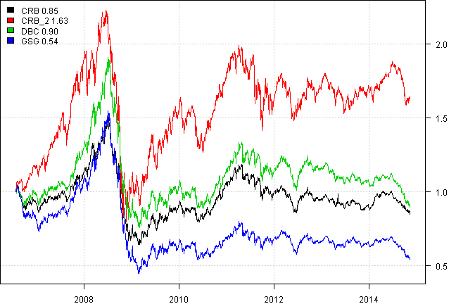
| CRB | CRB_2 | DBC | GSG | |
|---|---|---|---|---|
| CRB | 66% | 89% | 88% | |
| CRB_2 | 66% | 63% | ||
| DBC | 90% | |||
| Mean | -0.1% | 9.5% | 0.9% | -4.4% |
| StDev | 19.1% | 26.6% | 21.0% | 25.0% |
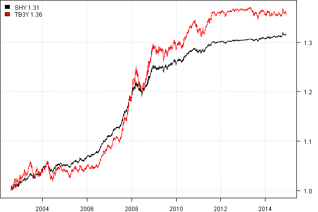
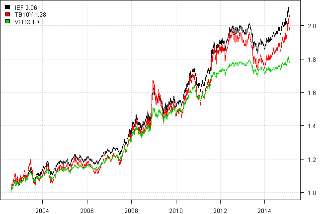
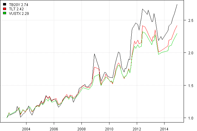
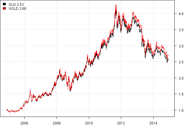
The historical commodity index data from crbequityindexes , that I denoted CRB_2, looks very different over the common interval for all proxies
proxy.overlay.plot(data)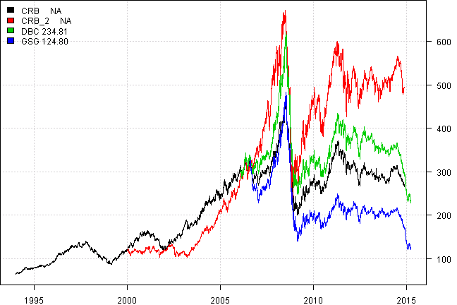
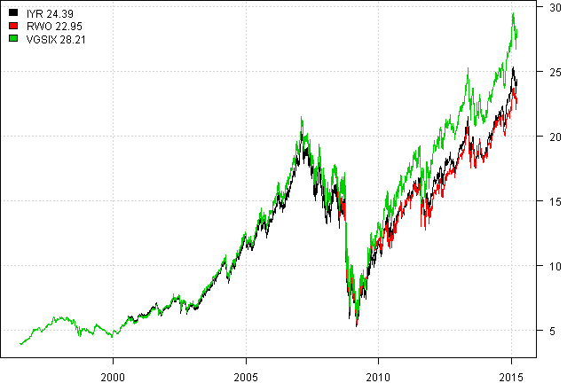
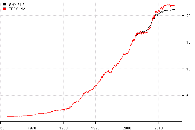
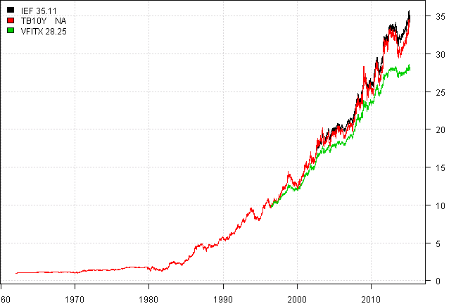
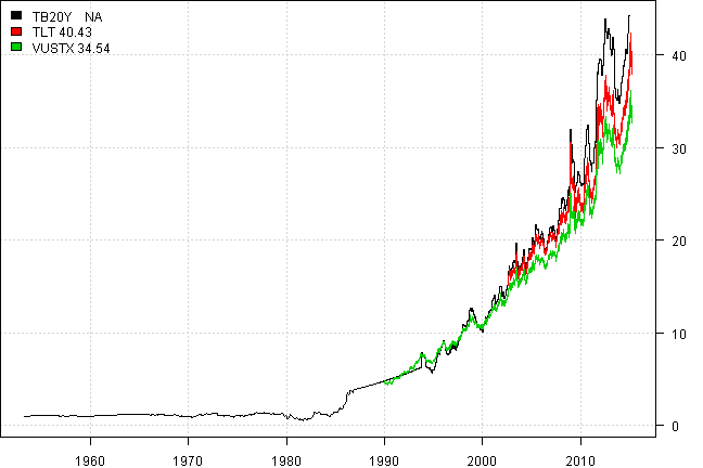
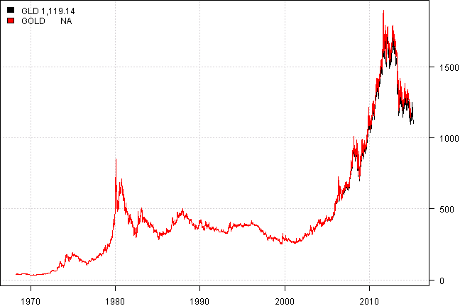
On the all history chart CRB_2 is also different.
proxy.prices(data) 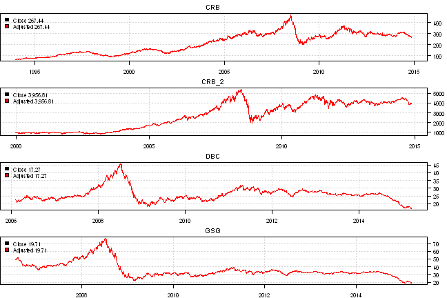
| CRB Price | CRB Total | CRB_2 Price | CRB_2 Total | DBC Price | DBC Total | GSG Price | GSG Total | |
|---|---|---|---|---|---|---|---|---|
| Mean | 8.2% | 8.2% | 11.5% | 11.5% | -0.8% | -0.8% | -7.5% | -7.5% |
| StDev | 16.3% | 16.3% | 21.5% | 21.5% | 20.9% | 20.9% | 25.0% | 25.0% |
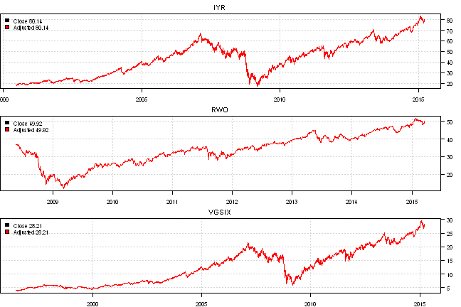
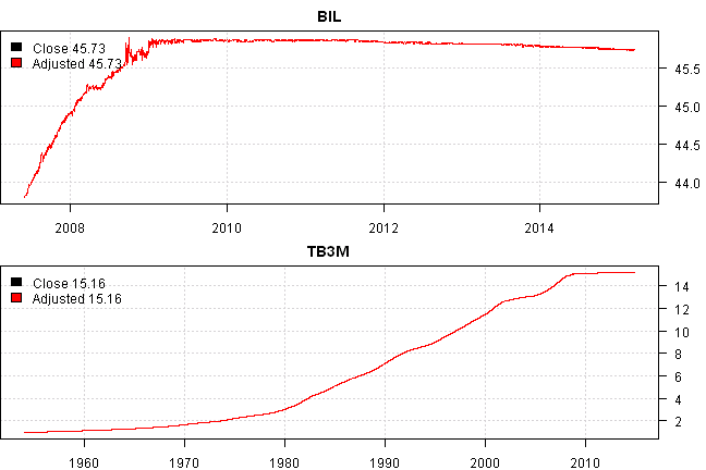
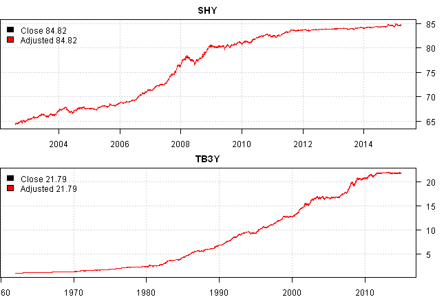
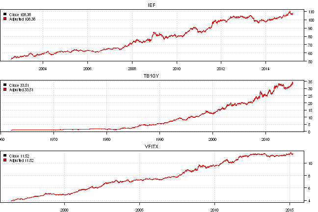
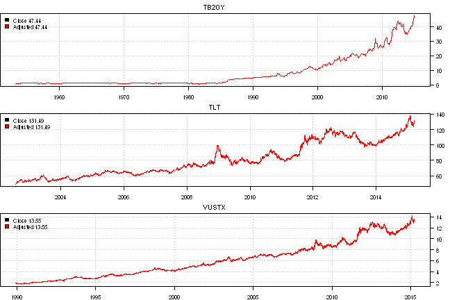
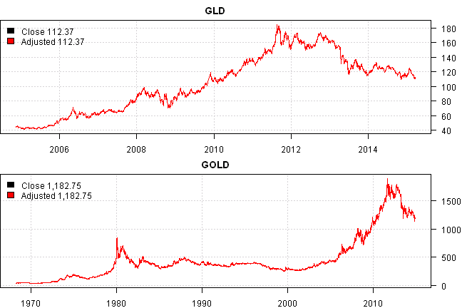
Quick glance at historical time series does not show anything abnormal between Price and Adjusted Price series.
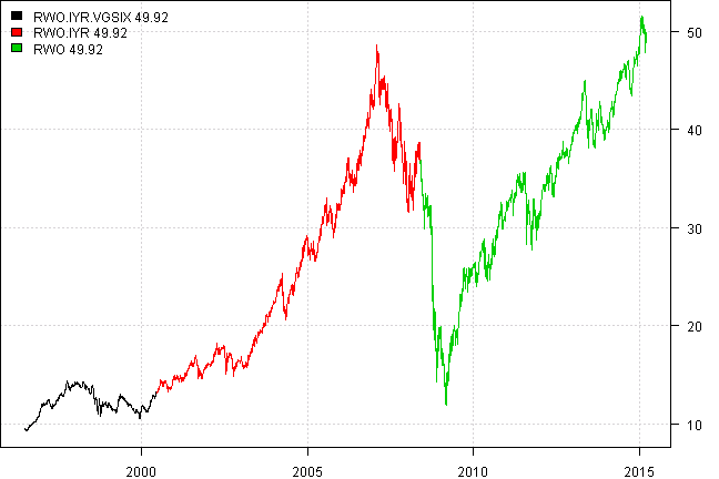
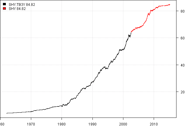
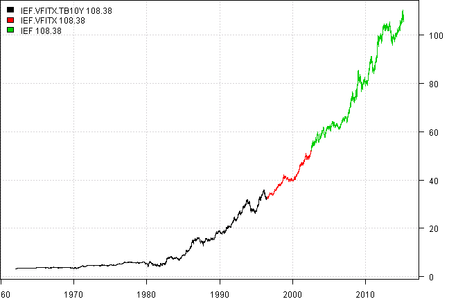
tickers = spl('DBC, DBC.CRB=DBC+CRB')
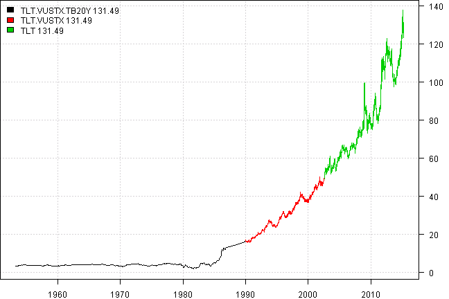
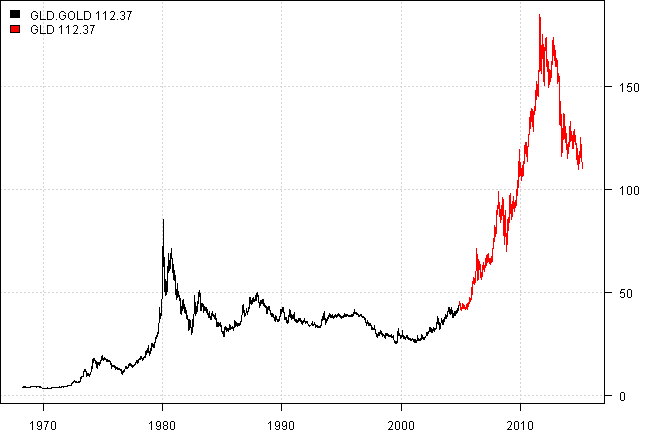
proxy.map(data, tickers) 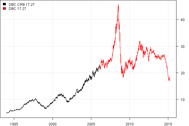
Please use CRB to extend Commodities.
REIT ex-U.S.:
(Dow Jones Global ex-U.S. Real Estate Securities Index)
create.proxy = function(tickers, proxy.map.tickers, raw.data = new.env()) {
    #*****************************************************************
    # Load historical data
    #******************************************************************
    load.packages('quantmod')

    tickers = spl(tickers)
    data = new.env()

    getSymbols.extra(tickers, src = 'yahoo', from = '1970-01-01', env = data, raw.data = raw.data, auto.assign = T)
        for(i in ls(data)) data[[i]] = adjustOHLC(data[[i]], use.Adjusted=T)

    #*****************************************************************
    # Compare
    #******************************************************************
    print(bt.start.dates(data))

    proxy.test(data)

    proxy.overlay.plot(data)

    proxy.prices(data)

    tickers = spl(proxy.map.tickers)
    proxy.map(data, tickers)
}

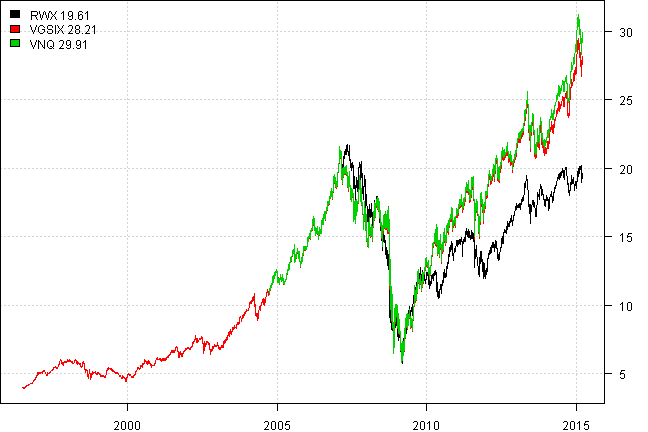
create.proxy('RWX,VNQ,VGSIX', 'RWX, RWX.VNQ=RWX+VNQ, RWX.VNQ.VGSIX=RWX+VNQ+VGSIX')| Start | |
|---|---|
| VGSIX | 1996-06-28 |
| VNQ | 2004-09-29 |
| RWX | 2007-03-02 |
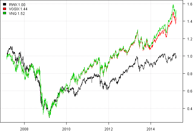
| RWX | VGSIX | VNQ | |
|---|---|---|---|
| RWX | 66% | 67% | |
| VGSIX | 99% | ||
| Mean | 3.3% | 12.6% | 12.9% |
| StDev | 25.4% | 40.2% | 39.1% |
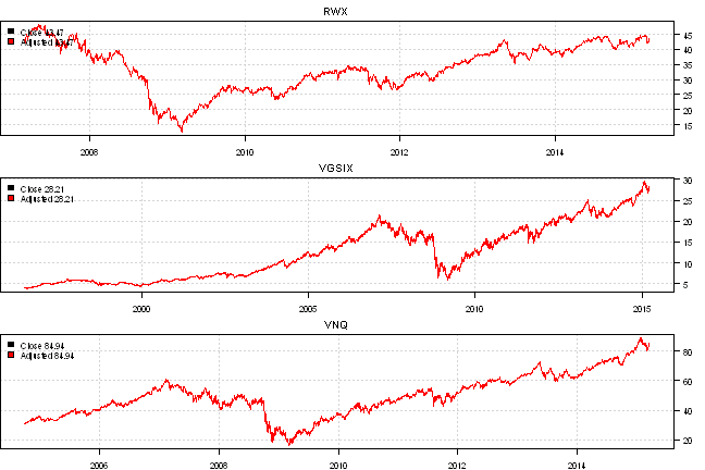
| RWX Price | RWX Total | VGSIX Price | VGSIX Total | VNQ Price | VNQ Total | |
|---|---|---|---|---|---|---|
| Mean | 3.3% | 3.3% | 14.4% | 14.4% | 15.9% | 15.9% |
| StDev | 25.4% | 25.4% | 28.1% | 28.1% | 35.1% | 35.1% |
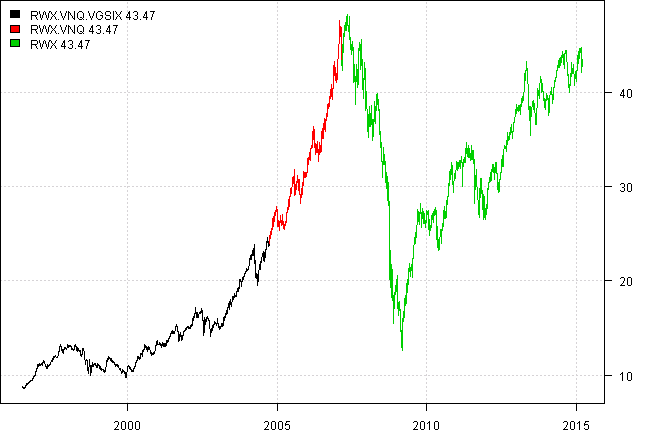
Please use VNQ and VGSIX to extend REIT ex-U.S.
Aside comparison of RWO vs. RWX: RWO vs. RWX: Head-To-Head ETF Comparison
Global REIT:
(Dow Jones Global Select Real Estate Securities Index)
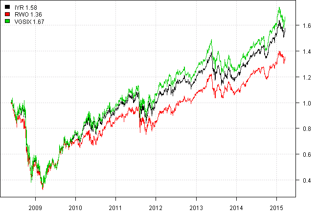
Please use IYR and VGSIX to extend Global REIT.
CASH:
GOLD:
	#--------------------------------
	# FTSE NAREIT U.S. Real Estate Index monthly total return series
	# http://returns.reit.com/returns/MonthlyHistoricalReturns.xls
	# https://r-forge.r-project.org/scm/viewvc.php/pkg/FinancialInstrument/inst/parser/download.NAREIT.R?view=markup&root=blotter
	filename = 'data/NAREIT.xls'
	if(!file.exists(filename)) {
		url = 'http://returns.reit.com/returns/MonthlyHistoricalReturns.xls'
		download.file(url, filename,  mode = 'wb')
	}

	load.packages('gdata')
	temp = read.xls(filename, pattern='Date', sheet='Index Data', stringsAsFactors=FALSE)
	index = as.numeric(gsub(',','',temp$Index))
	# monthly data, with 1-month-year format
	NAREIT = make.xts(index, as.Date(paste(1,temp$Date),'%d %b-%y'))
	raw.data$NAREIT = make.stock.xts(NAREIT)
	#--------------------------------
Let’s save these proxies in data.proxy.Rdata for convience to use later on
Syntax to specify tickers in getSymbols.extra function:
- Basic : XLY
- Rename: BOND=TLT
- Extend: XLB+RYBIX
- Mix above: XLB=XLB+RYBIX+FSDPX+FSCHX+PRNEX+DREVX
- TLT;MTM + IEF => TLT = TLT + IEF and MTM = MTM + IEF
- BOND = TLT;MTM + IEF => BOND = TLT + IEF, TLT = TLT + IEF, and MTM = MTM + IEF
- BOND;US.BOND = TLT;MTM + IEF => BOND = TLT + IEF, US.BOND = TLT + IEF, TLT = TLT + IEF, and MTM = MTM + IEF
-
BOND = [TLT] + IEF => BOND = TLT + IEF, and TLT = TLT + IEF
- use comma or new line to separate entries
- lines starting with
#symbol or empty lines are skipped Make sure not to use commas in comments
,message=T, warning=T
tickers = '
COM = DBC;GSG + CRB
RExUS = [RWX] + VNQ + VGSIX
RE = [RWX] + VNQ + VGSIX
RE.US = [ICF] + VGSIX
EMER.EQ = [EEM] + VEIEX
EMER.FI = [EMB] + PREMX
GOLD = [GLD] + GOLD,
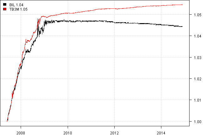
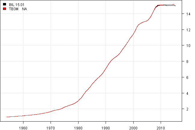
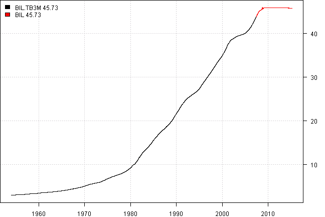
US.CASH = [BIL] + TB3M,
SHY + TB3Y,
US.HY = [HYG] + VWEHX
# Bonds
US.BOND = [AGG] + VBMFX
INTL.BOND = [BWX] + BEGBX
JAPAN.EQ = [EWJ] + FJPNX
EUROPE.EQ = [IEV] + FIEUX
US.SMCAP = IWM;VB + NAESX
TECH.EQ = [QQQ] + ^NDX
US.EQ = [VTI] + VTSMX + VFINX
US.MID = [VO] + VIMSX
EAFE = [EFA] + VDMIX + VGTSX
MID.TR = [IEF] + VFITX
CORP.FI = [LQD] + VWESX
TIPS = [TIP] + VIPSX + LSGSX
LONG.TR = [TLT] + VUSTX
'
data.proxy <- new.env()
getSymbols.extra(tickers, src = 'yahoo', from = '1970-01-01', env = data.proxy, raw.data = raw.data, auto.assign = T)
data.proxy.raw = raw.data
save(data.proxy.raw, file='data/data.proxy.raw.Rdata',compress='gzip')
save(data.proxy, file='data/data.proxy.Rdata',compress='gzip') To use saved proxy data to extend historical time series, use extend.data.proxy function:
tickers = spl('BIL')

data <- new.env()
getSymbols(tickers, src = 'yahoo', from = '1970-01-01', env = data, auto.assign = T)

print(bt.start.dates(data))| Start | |
|---|---|
| BIL | 2007-05-30 |
extend.data.proxy(data, proxy.filename = 'data/data.proxy.Rdata')

print(bt.start.dates(data))| Start | |
|---|---|
| BIL | 1954-01-04 |
(this report was produced on: 2015-03-19)