Country Seasonality
27 Mar 2016To install Systematic Investor Toolbox (SIT) please visit About page.
Meb Faber posted an interesting observation that if an asset or country is down 1/2/3 years in a row it historically recovers in the next 1/2 years. Details at 50% Returns Coming for Commodities and Emerging Markets? post.
The test of this simple strategy for historical country returns is below.
Load historical country returns from AQR data library
#*****************************************************************
# Read historical data from AQR library
# [Betting Against Beta: Equity Factors, Monthly](https://www.aqr.com/library/data-sets/betting-against-beta-equity-factors-monthly)
#******************************************************************
library(readxl)
library(SIT)
library(quantmod)

data = env()
data.set = 'betting-against-beta-equity-factors'

# monthly market returns in excess of t-bills
data$market.excess = load.aqr.data(data.set, 'monthly', 'MKT')

#monthly U.S. Treasury bill rates.
data$risk.free = load.aqr.data(data.set, 'monthly', 'RF', last.col2extract = 2)

# total market return
aqr.market = data$market.excess + as.vector(data$risk.free)

# compute equity
equity = bt.apply.matrix(1+ifna(aqr.market,0),cumprod)
	equity[is.na(aqr.market)] = NA

year.ends = date.ends(equity, 'year')

# create back-test environment with annual prices
data = env()
for(n in names(aqr.market))
	data[[n]] = make.stock.xts(equity[year.ends,n])
bt.prep(data, align='keep.all', fill.gaps = F, dates='1986::')

plota.matplot( scale.one(data$prices), main='Asset Performance')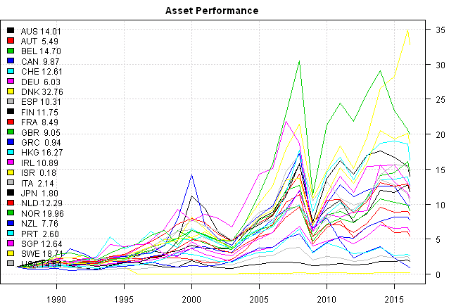
Look at historical stats for a strategy that invests in a country if is down 1/2/3 years in a row and holds for the next 1/2/3 years
#*****************************************************************
# Stats
#*****************************************************************
prices = data$prices
n = ncol(prices)
ret = prices / mlag(prices) - 1
signal = ret < 0
signals = list(down1yr = signal, down2yr = signal & mlag(signal), down3yr=signal & mlag(signal) & mlag(signal,2))
# compute stats
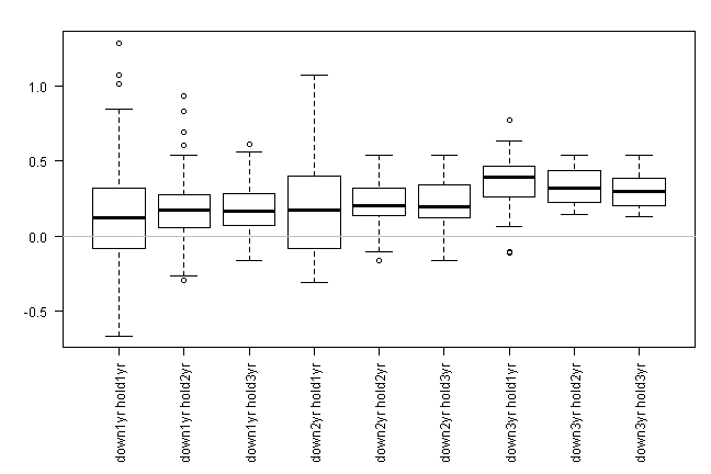
make.stats(signals, ret)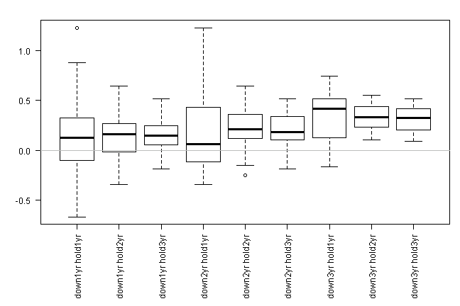
The least frequent the event, the better its historical performance. For example, after 3 years down there is on average a 30% bounce. After 2 years down there is on average a 20% bounce and after 1 year down there is on average a 15% bounce.
Next, create a strategy that invests in a country if is down 1/2/3 years in a row and holds for the next 1/2/3 years
#*****************************************************************
# Strategy
#*****************************************************************
models = run.models(signals, data)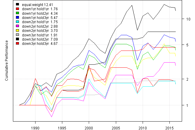
| equal.weight | down1yr hold1yr | down1yr hold2yr | down1yr hold3yr | down2yr hold1yr | down2yr hold2yr | down2yr hold3yr | down3yr hold1yr | down3yr hold2yr | down3yr hold3yr | |
|---|---|---|---|---|---|---|---|---|---|---|
| Period | Dec1986 - Feb2016 | Dec1986 - Feb2016 | Dec1986 - Feb2016 | Dec1986 - Feb2016 | Dec1986 - Feb2016 | Dec1986 - Feb2016 | Dec1986 - Feb2016 | Dec1986 - Feb2016 | Dec1986 - Feb2016 | Dec1986 - Feb2016 |
| Cagr | 9.01 | 1.96 | 5.16 | 6 | 1.94 | 3.69 | 4.59 | 2.24 | 6.94 | 5.42 |
| Sharpe | 0.5 | 0.18 | 0.33 | 0.36 | 0.17 | 0.24 | 0.28 | 0.22 | 0.4 | 0.32 |
| DVR | 0.44 | 0.03 | 0.24 | 0.29 | 0.09 | 0.19 | 0.24 | 0.2 | 0.37 | 0.29 |
| R2 | 0.88 | 0.19 | 0.75 | 0.81 | 0.52 | 0.76 | 0.85 | 0.89 | 0.92 | 0.89 |
| Volatility | 21.53 | 24.18 | 21.73 | 21.54 | 22.6 | 24.08 | 23.69 | 12.23 | 19.78 | 21.41 |
| MaxDD | -48.81 | -49.11 | -49.11 | -49.11 | -48.63 | -57.05 | -40.81 | -16.25 | -16.25 | -33.86 |
| Exposure | 96.77 | 70.97 | 83.87 | 90.32 | 48.39 | 64.52 | 77.42 | 22.58 | 35.48 | 48.39 |
| Win.Percent | 86.76 | 70.59 | 63.3 | 62.74 | 57.75 | 56.94 | 64 | 87.5 | 88 | 92.86 |
| Avg.Trade | 7.06 | 0.64 | 0.84 | 0.85 | 1.72 | 2.73 | 1.98 | 3.48 | 11.11 | 4.76 |
| Profit.Factor | 48.55 | 1.66 | 2.33 | 2.74 | 1.82 | 2.36 | 2.54 | 4.58 | 14.26 | 10.55 |
| Num.Trades | 68 | 204 | 297 | 314 | 71 | 72 | 100 | 24 | 25 | 42 |
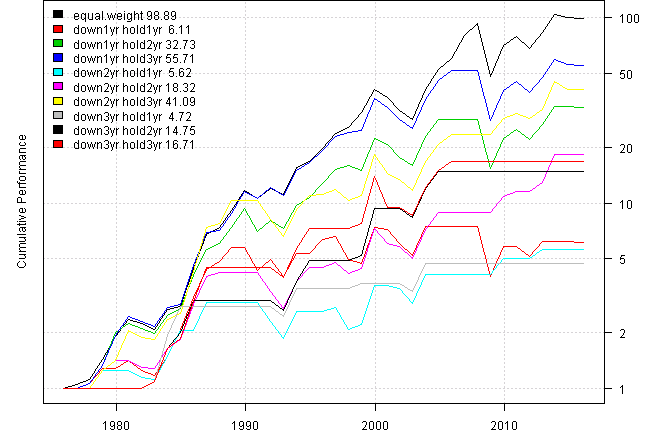
Please note that exposure, the time strategy is invested, is small, around 30%, for the least frequent the events, i.e. 3 years down.
Overall, it is hard to compete with always invested, equal weight, strategy because the timing signal, the number of years down, is not fully capturing all market movements.
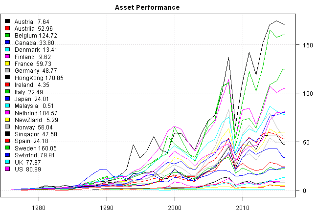
Below is the same analysis for country historical returns sourced form Kenneth R. French - Data Library](http://mba.tuck.dartmouth.edu/pages/faculty/ken.french/data_library.html)
| equal.weight | down1yr hold1yr | down1yr hold2yr | down1yr hold3yr | down2yr hold1yr | down2yr hold2yr | down2yr hold3yr | down3yr hold1yr | down3yr hold2yr | down3yr hold3yr | |
|---|---|---|---|---|---|---|---|---|---|---|
| Period | Dec1975 - Mar2016 | Dec1975 - Mar2016 | Dec1975 - Mar2016 | Dec1975 - Mar2016 | Dec1975 - Mar2016 | Dec1975 - Mar2016 | Dec1975 - Mar2016 | Dec1975 - Mar2016 | Dec1975 - Mar2016 | Dec1975 - Mar2016 |
| Cagr | 12.08 | 4.6 | 9.05 | 10.5 | 4.38 | 7.49 | 9.66 | 3.93 | 6.91 | 7.24 |
| Sharpe | 0.65 | 0.3 | 0.51 | 0.56 | 0.31 | 0.45 | 0.49 | 0.29 | 0.42 | 0.41 |
| DVR | 0.56 | 0.2 | 0.46 | 0.51 | 0.28 | 0.37 | 0.43 | 0.26 | 0.38 | 0.38 |
| R2 | 0.86 | 0.64 | 0.91 | 0.91 | 0.89 | 0.82 | 0.87 | 0.91 | 0.9 | 0.92 |
| Volatility | 21.15 | 21.64 | 21.12 | 21.65 | 17.94 | 19.6 | 23.29 | 16.21 | 18.87 | 21.34 |
| MaxDD | -48.26 | -46.21 | -46.21 | -46.21 | -35.66 | -35.66 | -36.12 | -11.53 | -11.53 | -38.97 |
| Exposure | 97.62 | 71.43 | 85.71 | 90.48 | 45.24 | 64.29 | 78.57 | 19.05 | 28.57 | 38.1 |
| Win.Percent | 87.42 | 64.56 | 67.27 | 72.21 | 62.5 | 62.92 | 70.69 | 90.48 | 91.3 | 88.89 |
| Avg.Trade | 5.78 | 1.16 | 3.21 | 4.48 | 4.39 | 9.44 | 15.87 | 13.96 | ||
| Profit.Factor | 39.63 | 1.96 | 2.65 | 3.83 | 5.03 | 10.07 | 17.71 | 17.03 | ||
| Num.Trades | 151 | 237 | 333 | 367 | 72 | 89 | 116 | 21 | 23 | 27 |
The results are similar to the results obtained using country historical returns sourced from AQR - Betting Against Beta: Equity Factors, Monthly data library.
These test were done based on absolute return being negative. The big question is if there is anything special about zero. I.e. is it significant to test against returns being below zero, or is it sufficient to test other values around zero.
For example, we may run the same tests using 1% as the trigger. Alternatively the trigger value can be derived from recent market data and adaptively adjusted as market enter new regimes.
#Supporting functions:
#*****************************************************************
# Stats
#*****************************************************************
make.stats = function(signals, ret) {
	# compute stats
	stats = list()
	for(signal in names(signals)) {
		temp = signals[[signal]]
		stats[[paste(signal,'hold1yr')]] = coredata(ret)[ifna(mlag(temp),F)]
		stats[[paste(signal,'hold2yr')]] = 1/2 * coredata(ret + mlag(ret,-1))[ifna(mlag(temp),F)]
		stats[[paste(signal,'hold3yr')]] = 1/3 * coredata(ret + mlag(ret,-1) + + mlag(ret,-3))[ifna(mlag(temp),F)]
	}
	stats = lapply(stats,na.omit)
	# sapply(stats,mean) # mean

	# make a barplot
	par(mar = c(8, 4, 2, 1))
	boxplot(stats,las=2)
		abline(h=0,col='gray')
}

#*****************************************************************
# Strategy
#*****************************************************************
run.models = function(signals, data) {
	models = list()

	data$weight[] = NA
		data$weight[] = ntop(prices, n)
	models$equal.weight = bt.run(data, trade.summary=T, silent=T)

	for(signal in names(signals)) {
		temp = signals[[signal]]
		data$weight[] = NA
			data$weight[] = ntop(temp, n)
		models[[paste(signal,'hold1yr')]] = bt.run(data, trade.summary=T, silent=T)

		temp = signals[[signal]]
			temp = temp | mlag(temp)
		data$weight[] = NA
			data$weight[] = ntop(temp, n)
		models[[paste(signal,'hold2yr')]] = bt.run(data, trade.summary=T, silent=T)

		temp = signals[[signal]]
			temp = temp | mlag(temp) | mlag(temp,2)
		data$weight[] = NA
			data$weight[] = ntop(temp, n)
		models[[paste(signal,'hold3yr')]] = bt.run(data, trade.summary=T, silent=T)
	}

	# create report
	plotbt(models, plotX = T, log = 'y', LeftMargin = 3, main = NULL)
		mtext('Cumulative Performance', side = 2, line = 1)

	print(plotbt.strategy.sidebyside(models, make.plot=F, return.table=T,perfromance.fn = engineering.returns.kpi))

	models
}
For your convenience, the 2016-03-27-Country-Seasonality post source code.