Channel Breakout - Second Attempt
09 Feb 2015To install Systematic Investor Toolbox (SIT) please visit About page.
David Varadi clarified the Channel Breakout system in the A ‘Simple’ Tactical Asset Allocation Portfolio with Percentile Channels (for Dummies) post.
Below I will try to adapt a code from the post:
#*****************************************************************
# Load historical data
#*****************************************************************
library(SIT)
load.packages('quantmod')

# load saved Proxies Raw Data, data.proxy.raw, to extend DBC and SHY
# please see http://systematicinvestor.github.io/Data-Proxy/ for more details
load('data/data.proxy.raw.Rdata')

tickers = '
LQD + VWESX
DBC + CRB
VTI +VTSMX # (or SPY)
ICF + VGSIX # (or IYR)
CASH = SHY + TB3Y
'

data <- new.env()
getSymbols.extra(tickers, src = 'yahoo', from = '1970-01-01', env = data, raw.data = data.proxy.raw, set.symbolnames = T, auto.assign = T)
for(i in data$symbolnames) data[[i]] = adjustOHLC(data[[i]], use.Adjusted=T)

#print(bt.start.dates(data))
bt.prep(data, align='remove.na', fill.gaps = T)

# Check data
plota.matplot(scale.one(data$prices),main='Asset Perfromance')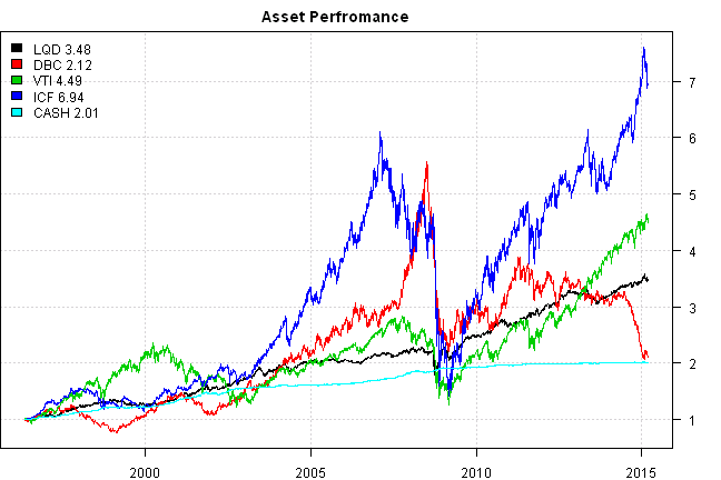
#*****************************************************************
# Setup
#*****************************************************************
data$universe = data$prices > 0
  # do not allocate to CASH, or BENCH
  data$universe$CASH = NA

prices = data$prices * data$universe
  n = ncol(prices)
  nperiods = nrow(prices)


frequency = 'months'
# find period ends, can be 'weeks', 'months', 'quarters', 'years'
period.ends = endpoints(prices, frequency)
  period.ends = period.ends[period.ends > 0]

models = list()

commission = list(cps = 0.01, fixed = 10.0, percentage = 0.0)

# lag prices by 1 day
#prices = mlag(prices)

#*****************************************************************
# Equal Weight each re-balancing period
#******************************************************************
data$weight[] = NA
  data$weight[period.ends,] = ntop(prices[period.ends,], n)
models$ew = bt.run.share(data, clean.signal=F, commission = commission, trade.summary=T, silent=T)

#*****************************************************************
# Risk Parity each re-balancing period
#******************************************************************
ret = diff(log(prices))
hist.vol = bt.apply.matrix(ret, runSD, n = 20)

# risk-parity
weight = 1 / hist.vol
rp.weight = weight / rowSums(weight, na.rm=T)

data$weight[] = NA
  data$weight[period.ends,] = rp.weight[period.ends,]
models$rp = bt.run.share(data, clean.signal=F, commission = commission, trade.summary=T, silent=T)

#*****************************************************************
# Strategy:
#
# 1) Use 60,120,180, 252-day percentile channels
# - corresponding to 3,6,9 and 12 months in the momentum literature-
# (4 separate systems) with a .75 long entry and .25 exit threshold with
# long triggered above .75 and holding through until exiting below .25
# (just like in the previous post) - no shorts!!!
#
# 2) If the indicator shows that you should be in cash, hold SHY
#
# 3) Use 20-day historical volatility for risk parity position-sizing
# among active assets (no leverage is used). This is 1/volatility (asset A)
# divided by the sum of 1/volatility for all assets to determine the position size.
#******************************************************************
allocation = 0 * ifna(prices, 0)
for(lockback.len in c(60,120,180, 252)) {
  high.channel = bt.apply.matrix(data$prices, runQuantile, lockback.len, probs=0.75)
  low.channel = bt.apply.matrix(data$prices, runQuantile, lockback.len, probs=0.25)
  signal = iif(cross.up(prices, high.channel), 1, iif(cross.dn(prices, low.channel), -1, NA))
  allocation = allocation + ifna( bt.apply.matrix(signal, ifna.prev), 0)
}

# (A) Channel score
allocation = ifna(allocation / 4, 0)

# equal-weight
weight = abs(allocation) / rowSums(abs(allocation))
	weight[allocation < 0] = 0
weight$CASH = 1 - rowSums(weight, na.rm=T)

data$weight[] = NA
  data$weight[period.ends,] = weight[period.ends,]
models$channel.ew = bt.run.share(data, clean.signal=F, commission = commission, trade.summary=T, silent=T)


# risk-parity: (C)
weight = allocation * 1 / hist.vol
weight = abs(weight) / rowSums(abs(weight), na.rm=T)
	weight[allocation < 0] = 0
weight$CASH = 1 - rowSums(weight, na.rm=T)

data$weight[] = NA
  data$weight[period.ends,] = ifna(weight[period.ends,], 0)
models$channel.rp = bt.run.share(data, clean.signal=F, commission = commission, trade.summary=T, silent=T)


# let's verify
last.period = last(period.ends)
print(allocation[last.period,])| LQD | DBC | VTI | ICF | CASH | |
|---|---|---|---|---|---|
| 2015-03-11 | 1 | -1 | 1 | 0.5 | 0 |
print(to.percent(last(hist.vol[last.period,])))| LQD | DBC | VTI | ICF | CASH | |
|---|---|---|---|---|---|
| 2015-03-11 | 0.45% | 0.94% | 0.60% | 1.28% |
print(to.percent(last(weight[last.period,])))| LQD | DBC | VTI | ICF | CASH | |
|---|---|---|---|---|---|
| 2015-03-11 | 41.59% | 0.00% | 31.27% | 7.30% | 19.85% |
Let’s add another benchmark, for comparison we will use the Quantitative Approach To Tactical Asset Allocation Strategy(QATAA) by Mebane T. Faber
#*****************************************************************
#The [Quantitative Approach To Tactical Asset Allocation Strategy(QATAA) by Mebane T. Faber](http://mebfaber.com/timing-model/)
#[SSRN paper](http://papers.ssrn.com/sol3/papers.cfm?abstract_id=962461)
#******************************************************************
# compute 10 month moving average
sma = bt.apply.matrix(prices, SMA, 200)

# go to cash if prices falls below 10 month moving average
go2cash = prices < sma
  go2cash = ifna(go2cash, T)

# equal weight target allocation
target.allocation = ntop(prices,n)

# If asset is above it's 10 month moving average it gets allocation
weight = iif(go2cash, 0, target.allocation)

# otherwise, it's weight is allocated to cash
weight$CASH = 1 - rowSums(weight)

data$weight[] = NA
  data$weight[period.ends,] = weight[period.ends,]
models$QATAA = bt.run.share(data, clean.signal=F, commission = commission, trade.summary=T, silent=T)


#*****************************************************************
# Report
#*****************************************************************
#strategy.performance.snapshoot(models, T)
plotbt(models, plotX = T, log = 'y', LeftMargin = 3, main = NULL)
	mtext('Cumulative Performance', side = 2, line = 1)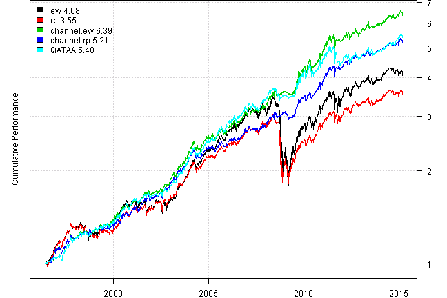
print(plotbt.strategy.sidebyside(models, make.plot=F, return.table=T))| ew | rp | channel.ew | channel.rp | QATAA | |
|---|---|---|---|---|---|
| Period | May1996 - Mar2015 | May1996 - Mar2015 | May1996 - Mar2015 | May1996 - Mar2015 | May1996 - Mar2015 |
| Cagr | 7.76 | 6.95 | 10.34 | 9.16 | 9.37 |
| Sharpe | 0.64 | 0.78 | 1.31 | 1.43 | 1.21 |
| DVR | 0.58 | 0.72 | 1.24 | 1.36 | 1.18 |
| Volatility | 13.13 | 9.19 | 7.76 | 6.28 | 7.64 |
| MaxDD | -48.78 | -40.52 | -11.55 | -6.98 | -13.71 |
| AvgDD | -1.51 | -1.22 | -1.26 | -1.11 | -1.05 |
| VaR | -1.07 | -0.76 | -0.74 | -0.59 | -0.71 |
| CVaR | -2 | -1.34 | -1.13 | -0.9 | -1.14 |
| Exposure | 99.7 | 99.28 | 99.7 | 99.7 | 99.7 |
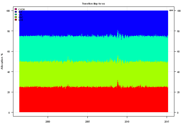
for(m in names(models)) {
print('#', m, 'strategy:')
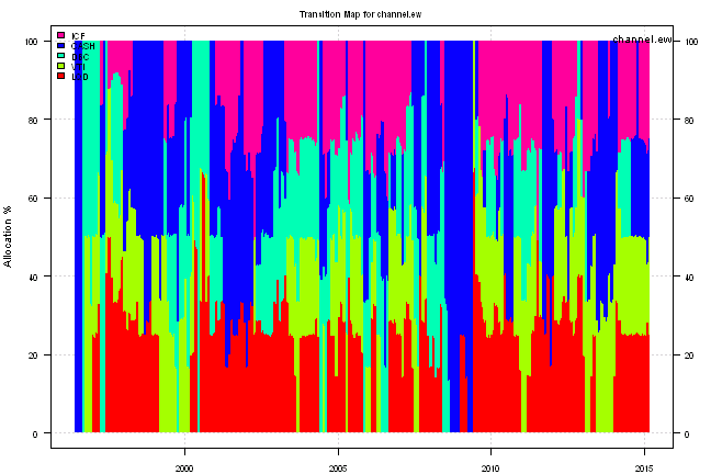
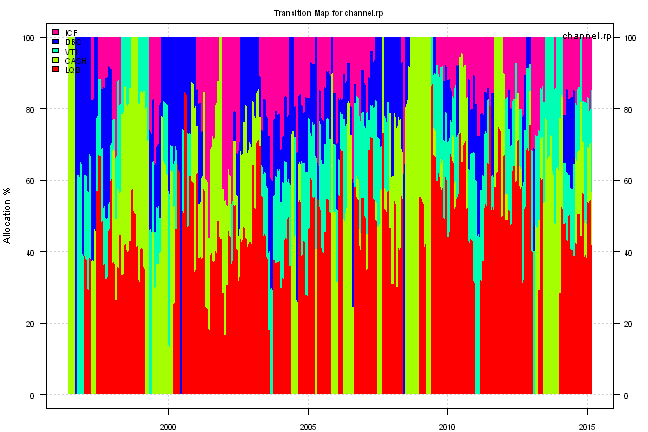
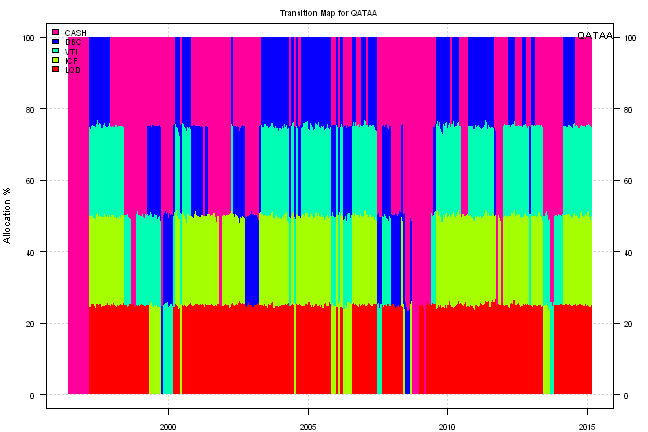
plotbt.transition.map(models[[m]]$weight, name=m)
legend('topright', legend = m, bty = 'n')
print(plotbt.monthly.table(models[[m]]$equity, make.plot = F))
print(to.percent(last(models[[m]]$weight)))
}ew strategy:
| Jan | Feb | Mar | Apr | May | Jun | Jul | Aug | Sep | Oct | Nov | Dec | Year | MaxDD | |
|---|---|---|---|---|---|---|---|---|---|---|---|---|---|---|
| 1996 | 1.3 | -1.6 | 2.8 | 3.0 | 1.6 | 5.0 | 2.5 | 15.3 | -3.2 | |||||
| 1997 | 1.4 | -0.4 | -1.0 | 1.1 | 3.4 | 1.8 | 4.8 | -1.6 | 4.9 | -0.7 | 0.1 | 0.3 | 14.7 | -4.9 |
| 1998 | -0.1 | 0.0 | 2.0 | -1.0 | -1.4 | 0.5 | -3.7 | -7.4 | 5.9 | -0.1 | 0.2 | 0.9 | -4.6 | -13.6 |
| 1999 | 0.4 | -3.3 | 4.3 | 4.2 | -1.5 | 2.3 | -1.5 | 0.9 | -0.3 | 0.2 | 1.2 | 3.2 | 10.2 | -4.9 |
| 2000 | 0.4 | 1.3 | 2.8 | -0.2 | 1.2 | 3.4 | 1.0 | 3.5 | -0.6 | -1.7 | -0.3 | 2.4 | 13.9 | -4.7 |
| 2001 | 1.8 | -2.8 | -2.8 | 3.3 | -0.1 | 0.1 | -0.2 | 0.1 | -5.5 | -0.5 | 3.0 | -0.2 | -3.9 | -11.3 |
| 2002 | -0.3 | 1.2 | 4.3 | -0.4 | 0.3 | -0.7 | -3.2 | 2.2 | -2.5 | 0.4 | 3.1 | 1.3 | 5.9 | -10.0 |
| 2003 | 0.4 | 2.0 | -1.3 | 3.2 | 4.8 | 0.8 | 1.0 | 2.3 | 1.4 | 2.2 | 1.7 | 4.1 | 24.9 | -3.4 |
| 2004 | 2.7 | 3.1 | 1.9 | -5.4 | 3.2 | -0.1 | 0.8 | 2.8 | 1.9 | 2.6 | 1.9 | 1.5 | 17.7 | -7.3 |
| 2005 | -2.1 | 2.8 | -0.2 | 0.0 | 1.6 | 2.3 | 4.0 | 0.5 | 0.1 | -2.7 | 2.4 | 1.8 | 10.8 | -4.4 |
| 2006 | 3.8 | -0.6 | 2.1 | 0.9 | -1.7 | 1.1 | 1.9 | 1.1 | 0.2 | 3.0 | 4.0 | -1.1 | 15.8 | -5.3 |
| 2007 | 2.3 | 0.6 | -0.6 | 1.7 | 0.1 | -3.2 | -2.5 | 2.1 | 4.7 | 3.0 | -3.5 | -0.1 | 4.3 | -7.8 |
| 2008 | -0.4 | 1.0 | 1.3 | 4.6 | 1.5 | -2.5 | -1.9 | -0.7 | -8.0 | -19.3 | -10.2 | 6.8 | -26.9 | -44.7 |
| 2009 | -8.2 | -11.3 | 4.0 | 11.5 | 6.9 | -0.9 | 6.1 | 3.9 | 3.3 | -0.3 | 4.9 | 1.8 | 21.1 | -24.9 |
| 2010 | -4.1 | 3.4 | 4.3 | 3.7 | -6.1 | -2.5 | 6.3 | -1.5 | 5.6 | 3.1 | -0.9 | 5.2 | 16.8 | -10.9 |
| 2011 | 2.4 | 3.4 | 0.2 | 3.9 | -0.8 | -2.6 | 1.6 | -2.9 | -8.4 | 9.1 | -2.0 | 1.5 | 4.4 | -14.8 |
| 2012 | 4.2 | 2.4 | 1.2 | 0.4 | -5.3 | 3.0 | 3.1 | 2.0 | 0.2 | -1.4 | 0.3 | 0.8 | 11.1 | -7.5 |
| 2013 | 2.3 | -0.6 | 1.7 | 1.7 | -2.2 | -2.3 | 2.5 | -2.0 | 1.0 | 2.4 | -1.0 | 0.9 | 4.3 | -7.9 |
| 2014 | 0.0 | 4.0 | 0.3 | 1.6 | 1.1 | 1.3 | -1.7 | 1.9 | -4.3 | 2.7 | -0.7 | -2.0 | 4.1 | -5.6 |
| 2015 | 0.6 | 1.1 | -2.6 | -0.9 | -3.4 | |||||||||
| Avg | 0.4 | 0.4 | 1.2 | 1.9 | 0.3 | 0.2 | 0.9 | 0.5 | 0.2 | 0.2 | 0.5 | 1.7 | 7.9 | -10.0 |
| LQD | DBC | VTI | ICF | CASH | |
|---|---|---|---|---|---|
| 2015-03-11 | 25.37% | 24.47% | 25.06% | 25.10% | 0.00% |
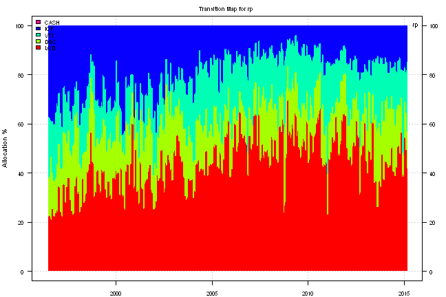
rp strategy:
| Jan | Feb | Mar | Apr | May | Jun | Jul | Aug | Sep | Oct | Nov | Dec | Year | MaxDD | |
|---|---|---|---|---|---|---|---|---|---|---|---|---|---|---|
| 1996 | -0.1 | -1.5 | 3.0 | 2.9 | 2.0 | 5.0 | 3.1 | 15.1 | -3.2 | |||||
| 1997 | 1.0 | -0.3 | -0.7 | 1.0 | 2.9 | 2.2 | 4.7 | -1.5 | 5.4 | -0.7 | -0.5 | 0.2 | 14.3 | -4.7 |
| 1998 | -0.1 | -0.7 | 2.1 | -0.9 | -1.1 | 0.6 | -3.3 | -5.0 | 4.9 | -1.5 | -1.2 | 0.5 | -5.8 | -10.3 |
| 1999 | 0.2 | -3.1 | 3.1 | 3.9 | -1.5 | 1.6 | -1.6 | 0.4 | -0.3 | -0.6 | 0.3 | 2.3 | 4.4 | -4.8 |
| 2000 | 0.4 | 1.1 | 2.6 | 1.0 | 1.2 | 3.0 | 1.2 | 2.1 | -0.3 | -1.2 | 1.2 | 3.2 | 16.4 | -3.5 |
| 2001 | 1.8 | -1.7 | -1.9 | 1.6 | -0.2 | 1.2 | 0.3 | 1.2 | -4.6 | 0.5 | 2.2 | 0.2 | 0.5 | -7.9 |
| 2002 | -0.2 | 1.4 | 2.8 | 0.2 | 0.6 | 0.1 | -2.5 | 3.1 | -0.3 | -1.0 | 2.0 | 2.4 | 8.9 | -7.5 |
| 2003 | -0.5 | 2.3 | -0.4 | 2.6 | 4.5 | 0.5 | -0.2 | 2.3 | 1.8 | 1.4 | 1.5 | 3.6 | 21.1 | -2.6 |
| 2004 | 2.7 | 2.3 | 1.4 | -5.5 | 1.9 | 0.0 | 0.5 | 2.4 | 1.4 | 2.3 | 1.3 | 1.5 | 12.7 | -7.4 |
| 2005 | -1.6 | 1.5 | -0.7 | -0.2 | 1.5 | 1.8 | 3.1 | 0.7 | -0.7 | -2.2 | 1.5 | 1.6 | 6.3 | -3.7 |
| 2006 | 2.6 | -0.2 | 0.3 | 0.6 | -1.3 | 0.4 | 1.8 | 1.6 | 0.8 | 2.4 | 3.1 | -0.7 | 11.9 | -3.3 |
| 2007 | 1.4 | 0.5 | -0.6 | 1.3 | -0.1 | -1.5 | -1.7 | 1.8 | 4.0 | 2.7 | -2.1 | 0.1 | 5.8 | -4.8 |
| 2008 | 0.4 | 1.1 | 0.2 | 3.2 | 0.6 | -3.1 | -0.9 | -0.6 | -9.6 | -19.1 | -6.3 | 9.8 | -24.1 | -40.0 |
| 2009 | -4.6 | -7.9 | 2.6 | 5.6 | 5.1 | 0.8 | 5.5 | 2.5 | 2.4 | -0.3 | 3.8 | -0.3 | 15.2 | -17.2 |
| 2010 | -2.5 | 2.1 | 2.9 | 2.9 | -4.5 | 0.3 | 4.1 | 0.7 | 4.2 | 2.3 | -1.1 | 3.5 | 15.2 | -6.2 |
| 2011 | 2.1 | 2.7 | 0.0 | 3.3 | 0.1 | -1.6 | 1.8 | -1.9 | -5.9 | 5.6 | -2.5 | 2.2 | 5.4 | -9.3 |
| 2012 | 3.5 | 2.3 | 0.2 | 0.5 | -3.5 | 2.2 | 3.2 | 0.9 | 0.4 | -0.6 | -0.1 | 0.3 | 9.4 | -4.8 |
| 2013 | 1.3 | -0.1 | 0.9 | 2.1 | -2.8 | -2.5 | 2.5 | -1.2 | 0.7 | 2.4 | -0.6 | 0.9 | 3.5 | -7.2 |
| 2014 | 0.0 | 3.2 | 0.2 | 1.4 | 1.1 | 1.0 | -1.6 | 1.7 | -3.4 | 1.7 | 0.0 | -0.7 | 4.6 | -4.4 |
| 2015 | 1.9 | 0.0 | -2.1 | -0.3 | -3.1 | |||||||||
| Avg | 0.5 | 0.3 | 0.7 | 1.4 | 0.2 | 0.4 | 0.8 | 0.7 | 0.2 | -0.2 | 0.4 | 1.8 | 7.0 | -7.8 |
| LQD | DBC | VTI | ICF | CASH | |
|---|---|---|---|---|---|
| 2015-03-11 | 42.33% | 14.48% | 28.40% | 14.80% | 0.00% |
channel.ew strategy:
| Jan | Feb | Mar | Apr | May | Jun | Jul | Aug | Sep | Oct | Nov | Dec | Year | MaxDD | |
|---|---|---|---|---|---|---|---|---|---|---|---|---|---|---|
| 1996 | 0.9 | 0.3 | -0.1 | 1.5 | 0.4 | 6.2 | 1.1 | 10.6 | -2.3 | |||||
| 1997 | 1.5 | -0.7 | -1.5 | 0.5 | 1.7 | 0.8 | 6.1 | -2.1 | 3.7 | 0.0 | -0.9 | 0.3 | 9.6 | -4.9 |
| 1998 | 0.5 | 1.5 | 1.9 | 0.1 | 0.0 | 1.3 | -0.6 | -2.6 | 2.4 | -0.4 | 0.3 | 1.9 | 6.5 | -4.2 |
| 1999 | 1.4 | -2.5 | 1.8 | 2.3 | -1.6 | 2.6 | -1.2 | 1.0 | 0.7 | -1.1 | 1.9 | 2.9 | 8.2 | -4.2 |
| 2000 | 0.3 | 1.8 | 1.9 | -2.8 | 3.6 | 3.5 | -1.5 | 4.1 | -1.7 | -0.5 | 2.4 | 1.1 | 12.7 | -6.9 |
| 2001 | 1.5 | 0.1 | -0.5 | -0.2 | 0.7 | 2.6 | 1.2 | 2.1 | -0.1 | 1.4 | -1.4 | -0.2 | 7.2 | -3.6 |
| 2002 | 0.1 | 1.1 | 0.2 | -0.3 | 1.0 | 1.3 | -0.5 | 2.3 | 1.7 | -0.2 | 0.1 | 3.8 | 10.9 | -4.1 |
| 2003 | 3.0 | 2.3 | -2.6 | 1.3 | 4.7 | 0.8 | 1.0 | 2.4 | 0.4 | 2.2 | 1.7 | 4.1 | 23.2 | -4.7 |
| 2004 | 2.7 | 3.1 | 1.9 | -5.9 | 2.3 | -2.1 | -0.1 | 3.3 | 1.7 | 2.6 | 1.9 | 1.5 | 13.1 | -7.0 |
| 2005 | -2.8 | 2.9 | -0.1 | -3.5 | 1.2 | 2.3 | 4.0 | 0.5 | 0.1 | -3.2 | 0.1 | 1.2 | 2.5 | -5.9 |
| 2006 | 4.7 | -0.7 | 2.0 | 1.0 | -1.6 | 0.8 | 2.1 | 0.2 | 0.9 | 3.2 | 2.8 | -1.1 | 15.0 | -5.3 |
| 2007 | 2.3 | -0.8 | -0.8 | 1.4 | 0.3 | -0.4 | -0.1 | 0.1 | 0.6 | 3.2 | -1.4 | 1.4 | 5.7 | -5.9 |
| 2008 | 2.2 | 3.0 | -0.3 | 1.8 | 1.4 | 3.3 | -3.0 | -0.6 | 0.5 | 1.1 | 1.1 | 0.5 | 11.2 | -5.4 |
| 2009 | -0.8 | -1.4 | 0.5 | -0.2 | 0.0 | 2.0 | 3.7 | 4.9 | 4.4 | -2.3 | 4.9 | 1.8 | 18.5 | -5.4 |
| 2010 | -4.1 | 3.3 | 4.8 | 3.2 | -6.1 | 0.4 | 2.2 | 0.6 | 1.3 | 3.1 | -1.0 | 6.3 | 13.9 | -9.6 |
| 2011 | 3.2 | 4.1 | 0.3 | 4.1 | -0.8 | -2.4 | 2.1 | -2.5 | 0.0 | 0.6 | -1.3 | 0.6 | 8.2 | -11.5 |
| 2012 | 2.0 | 1.2 | 1.6 | 0.7 | -3.4 | 1.8 | 1.9 | 0.6 | 0.2 | -1.5 | 0.4 | -0.2 | 5.4 | -5.8 |
| 2013 | 3.0 | -1.1 | 2.1 | 2.8 | -1.9 | -1.0 | 1.5 | -1.1 | 1.3 | 1.2 | 0.0 | 0.8 | 7.7 | -6.4 |
| 2014 | -0.6 | 1.9 | 0.3 | 1.6 | 1.1 | 1.3 | -1.7 | 2.3 | -2.5 | 1.1 | 1.5 | 0.3 | 6.8 | -3.2 |
| 2015 | 2.2 | -0.9 | -1.5 | -0.3 | -3.6 | |||||||||
| Avg | 1.2 | 0.9 | 0.6 | 0.4 | 0.1 | 1.0 | 0.9 | 0.8 | 0.9 | 0.6 | 1.0 | 1.5 | 9.8 | -5.5 |
| LQD | DBC | VTI | ICF | CASH | |
|---|---|---|---|---|---|
| 2015-03-11 | 25.06% | 0.00% | 24.76% | 24.79% | 25.39% |
channel.rp strategy:
| Jan | Feb | Mar | Apr | May | Jun | Jul | Aug | Sep | Oct | Nov | Dec | Year | MaxDD | |
|---|---|---|---|---|---|---|---|---|---|---|---|---|---|---|
| 1996 | 0.9 | 0.3 | -0.1 | 1.5 | 0.6 | 6.3 | 0.9 | 10.6 | -2.2 | |||||
| 1997 | 1.3 | -0.6 | -1.4 | 0.4 | 1.7 | 1.1 | 5.8 | -2.0 | 3.8 | 0.2 | -1.3 | 0.4 | 9.4 | -4.7 |
| 1998 | 0.6 | 0.5 | 1.9 | -0.1 | 0.3 | 1.3 | -0.6 | -0.9 | 2.7 | -1.0 | 0.6 | 1.5 | 6.9 | -4.0 |
| 1999 | 1.2 | -2.6 | 1.3 | 1.3 | -1.6 | 1.9 | -1.3 | 0.5 | 0.7 | -0.9 | 1.2 | 1.8 | 3.6 | -4.1 |
| 2000 | 0.3 | 1.6 | 1.5 | -2.1 | 2.0 | 3.5 | -0.8 | 2.6 | -1.3 | -0.1 | 2.0 | 1.3 | 10.9 | -4.7 |
| 2001 | 1.9 | 0.0 | -0.4 | -0.5 | 0.7 | 3.5 | 1.3 | 2.3 | -0.2 | 2.1 | -1.6 | 0.1 | 9.5 | -3.8 |
| 2002 | 0.1 | 1.4 | 0.3 | 0.4 | 1.1 | 1.1 | -1.2 | 3.1 | 1.9 | -0.3 | 0.4 | 3.8 | 12.7 | -5.1 |
| 2003 | 0.9 | 2.3 | -1.2 | 1.8 | 4.4 | 0.5 | -0.2 | 2.4 | 0.7 | 1.4 | 1.5 | 3.6 | 19.6 | -3.7 |
| 2004 | 2.7 | 2.3 | 1.4 | -5.9 | 1.8 | -1.5 | -0.4 | 2.7 | 1.2 | 2.3 | 1.3 | 1.5 | 9.7 | -7.0 |
| 2005 | -1.9 | 1.3 | -0.6 | -2.5 | 1.3 | 1.7 | 3.1 | 0.7 | -0.7 | -2.4 | 0.3 | 1.0 | 1.0 | -4.9 |
| 2006 | 3.7 | -0.2 | 0.0 | 0.8 | -1.2 | 0.4 | 1.4 | 0.3 | 1.0 | 2.4 | 2.6 | -0.7 | 11.1 | -2.6 |
| 2007 | 1.4 | -0.4 | -0.7 | 1.1 | 0.1 | -0.8 | 0.1 | 0.1 | 0.6 | 2.8 | -0.8 | 1.0 | 4.3 | -3.5 |
| 2008 | 2.4 | 2.1 | -0.4 | 1.5 | 0.2 | 2.2 | -1.5 | -0.2 | 0.5 | 1.1 | 1.1 | 0.5 | 9.7 | -3.9 |
| 2009 | -1.2 | -2.9 | 0.5 | -0.2 | 0.0 | 2.5 | 4.4 | 3.0 | 3.0 | -1.4 | 3.8 | -0.3 | 11.4 | -5.8 |
| 2010 | -2.5 | 1.8 | 2.8 | 2.5 | -4.6 | 2.1 | 1.9 | 1.9 | 0.9 | 2.3 | -1.1 | 4.8 | 13.0 | -6.1 |
| 2011 | 2.8 | 4.0 | 0.1 | 3.6 | 0.1 | -1.5 | 2.3 | -1.5 | 0.1 | 1.5 | -2.4 | 1.7 | 11.2 | -6.9 |
| 2012 | 2.0 | 1.6 | 0.4 | 0.7 | -1.6 | 1.3 | 2.8 | 0.3 | 0.4 | -0.5 | -0.2 | -0.3 | 7.1 | -4.0 |
| 2013 | 1.8 | -0.8 | 1.6 | 2.8 | -2.6 | -0.8 | 1.4 | -1.1 | 1.2 | 1.6 | 0.2 | 0.9 | 6.2 | -5.2 |
| 2014 | -0.1 | 1.3 | 0.2 | 1.4 | 1.1 | 1.0 | -1.6 | 2.0 | -2.1 | 1.1 | 1.2 | 0.2 | 5.8 | -2.2 |
| 2015 | 2.9 | -1.3 | -1.5 | 0.0 | -3.1 | |||||||||
| Avg | 1.1 | 0.6 | 0.3 | 0.4 | 0.2 | 1.1 | 0.9 | 0.9 | 0.8 | 0.7 | 0.8 | 1.2 | 8.7 | -4.4 |
| LQD | DBC | VTI | ICF | CASH | |
|---|---|---|---|---|---|
| 2015-03-11 | 42.02% | 0.00% | 28.19% | 14.69% | 15.09% |
QATAA strategy:
| Jan | Feb | Mar | Apr | May | Jun | Jul | Aug | Sep | Oct | Nov | Dec | Year | MaxDD | |
|---|---|---|---|---|---|---|---|---|---|---|---|---|---|---|
| 1996 | 0.9 | 0.3 | 0.1 | 1.2 | 1.5 | 1.1 | -0.5 | 4.6 | -1.0 | |||||
| 1997 | 0.4 | -0.1 | -1.0 | 1.1 | 3.4 | 1.8 | 4.8 | -1.6 | 4.9 | -0.7 | 0.1 | 1.6 | 15.4 | -4.9 |
| 1998 | 0.4 | 1.3 | 2.0 | -0.3 | -0.3 | 1.5 | -0.6 | -2.6 | 2.4 | -0.3 | 1.8 | 1.9 | 7.3 | -4.2 |
| 1999 | 1.4 | -2.5 | 1.3 | 1.8 | -1.2 | 2.6 | -1.2 | 1.0 | -0.4 | -1.0 | 1.7 | 2.5 | 6.0 | -3.2 |
| 2000 | 0.0 | 1.8 | 2.2 | -0.2 | 1.2 | 3.0 | 1.0 | 3.5 | -0.6 | -1.7 | 2.5 | 2.4 | 16.0 | -4.7 |
| 2001 | 1.2 | -0.2 | -1.0 | 0.1 | -0.2 | 1.8 | 1.2 | 2.1 | -0.1 | 0.8 | -1.3 | -0.2 | 4.1 | -3.7 |
| 2002 | 0.3 | 1.0 | -0.3 | -0.4 | 0.9 | 1.4 | -0.5 | 2.2 | 0.2 | -0.2 | 0.1 | 3.1 | 7.8 | -3.3 |
| 2003 | 1.8 | 2.0 | -1.9 | 1.0 | 4.8 | 0.8 | 1.0 | 2.3 | 1.4 | 2.2 | 1.7 | 4.1 | 23.3 | -3.7 |
| 2004 | 2.7 | 3.1 | 1.9 | -5.5 | 1.2 | -0.1 | 0.4 | 2.7 | 1.5 | 2.6 | 1.9 | 1.5 | 14.5 | -6.5 |
| 2005 | -2.1 | 2.8 | -0.2 | 0.0 | 1.6 | 2.3 | 4.0 | 0.5 | 0.1 | -2.8 | 2.3 | 1.6 | 10.6 | -4.4 |
| 2006 | 3.8 | -0.7 | 2.1 | 1.0 | -1.6 | 1.2 | 1.7 | 1.1 | 0.2 | 2.9 | 2.5 | -1.1 | 13.7 | -5.3 |
| 2007 | 2.3 | -0.5 | -0.6 | 1.7 | 0.1 | -3.2 | 0.0 | 0.4 | 3.6 | 2.9 | -0.6 | 1.2 | 7.3 | -5.4 |
| 2008 | 2.2 | 3.0 | -0.4 | 1.4 | 0.9 | -0.2 | -2.1 | -1.3 | -2.7 | 1.1 | 1.1 | 0.5 | 3.3 | -9.5 |
| 2009 | -0.8 | -1.4 | 0.5 | 0.6 | 0.6 | 0.7 | 3.5 | 3.9 | 3.3 | -0.3 | 4.9 | 1.8 | 18.3 | -5.1 |
| 2010 | -4.1 | 2.4 | 4.3 | 3.7 | -6.1 | -1.9 | 3.2 | 0.6 | 1.1 | 3.1 | -0.9 | 5.2 | 10.2 | -10.0 |
| 2011 | 2.4 | 3.4 | 0.2 | 3.9 | -0.8 | -2.6 | 1.6 | -2.9 | -6.5 | 0.6 | -1.8 | 0.9 | -2.2 | -13.7 |
| 2012 | 3.3 | 1.0 | 1.2 | 0.4 | -5.3 | 2.5 | 1.7 | 0.5 | 0.2 | -1.5 | -0.2 | -0.1 | 3.5 | -7.2 |
| 2013 | 2.3 | -0.6 | 1.6 | 2.7 | -1.9 | -0.8 | 1.5 | -2.5 | 1.1 | 1.1 | 0.7 | 0.6 | 5.8 | -6.0 |
| 2014 | -0.2 | 1.5 | 0.3 | 1.6 | 1.1 | 1.3 | -1.7 | 2.3 | -2.5 | 3.7 | 1.5 | 0.3 | 9.3 | -2.7 |
| 2015 | 2.2 | -0.1 | -1.5 | 0.5 | -2.8 | |||||||||
| Avg | 1.0 | 0.9 | 0.6 | 0.8 | -0.1 | 0.7 | 1.0 | 0.6 | 0.4 | 0.7 | 1.0 | 1.4 | 9.0 | -5.4 |
| LQD | DBC | VTI | ICF | CASH | |
|---|---|---|---|---|---|
| 2015-03-11 | 25.06% | 0.00% | 24.76% | 24.79% | 25.39% |
# plotbt(models[3], xfun = function(x) { 100 * compute.drawdown(x$equity) })Finnally, let’s zoom in on the recent perfomance strating in 2010:
models.2010 = bt.trim(models, dates = '2010::')

plotbt(models.2010, plotX = T, log = 'y', LeftMargin = 3, main = NULL)
	mtext('Cumulative Performance', side = 2, line = 1)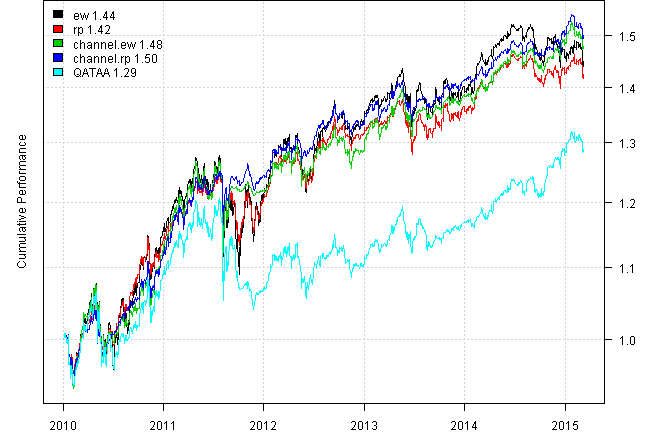
print(plotbt.strategy.sidebyside(models.2010, make.plot=F, return.table=T))| ew | rp | channel.ew | channel.rp | QATAA | |
|---|---|---|---|---|---|
| Period | Jan2010 - Mar2015 | Jan2010 - Mar2015 | Jan2010 - Mar2015 | Jan2010 - Mar2015 | Jan2010 - Mar2015 |
| Cagr | 7.33 | 6.99 | 7.79 | 8.1 | 4.97 |
| Sharpe | 0.69 | 0.96 | 0.92 | 1.27 | 0.6 |
| DVR | 0.64 | 0.89 | 0.86 | 1.2 | 0.44 |
| Volatility | 11.42 | 7.57 | 8.82 | 6.47 | 9.12 |
| MaxDD | -14.76 | -9.27 | -11.55 | -6.91 | -13.71 |
| AvgDD | -1.64 | -1.2 | -1.57 | -1.12 | -1.57 |
| VaR | -1.12 | -0.73 | -0.82 | -0.59 | -0.92 |
| CVaR | -1.75 | -1.13 | -1.38 | -1 | -1.45 |
| Exposure | 100 | 100 | 100 | 100 | 100 |
We are able to match the sharpe ratio of about 1.5 using ETF data as reported in the source source
Thank you David for this concept; it is a very robust allocation framework.
(this report was produced on: 2015-03-12)