Channel Breakout
02 Feb 2015To install Systematic Investor Toolbox (SIT) please visit About page.
David Varadi did a few posts on Channel Breakout systems:
- Percentile Channels: A New Twist On a Trend-Following Favorite
- A Simple Tactical Asset Allocation Portfolio with Percentile Channels
Below I will try to adapt a code from the posts:
#*****************************************************************
# First, reproduce S&P 500 chart
#*****************************************************************
library(SIT)
load.packages('quantmod')
tickers = 'SP=^GSPC'

data <- new.env()
getSymbols.extra(tickers, src = 'yahoo', from = '1970-01-01', env = data, auto.assign = T)
for(i in ls(data)) data[[i]] = adjustOHLC(data[[i]], use.Adjusted=T)

# compute Donchian channels
d.high.channel = runMax(Hi(data$SP), 55)
d.low.channel = runMin(Lo(data$SP), 55)

# compute Percentile channels
p.high.channel = runQuantile(Cl(data$SP), 55, probs=0.75)
p.low.channel = runQuantile(Cl(data$SP), 55, probs=0.25)

# compute Average
sma = SMA(Cl(data$SP), 55)

# make plot
plota(data$SP['2013:10::2014',],type='l', col='lightblue', lwd=2)
  plota.legend('SP')
plota.lines(sma, col='green', lwd=2)
plota.lines(d.high.channel, col='red', lwd=2)
plota.lines(d.low.channel, col='gray', lwd=2)
plota.lines(p.high.channel, col='yellow', lwd=2)
plota.lines(p.low.channel, col='blue', lwd=2)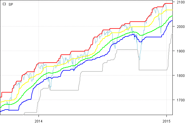
#*****************************************************************
# Load historical data
#*****************************************************************
library(SIT)
load.packages('quantmod')
tickers = 'DBC+CRB'

# load saved Proxies Raw Data, data.proxy.raw
# please see http://systematicinvestor.github.io/Data-Proxy/ for more details
load('data/data.proxy.raw.Rdata')

data <- new.env()
getSymbols.extra(tickers, src = 'yahoo', from = '1970-01-01', env = data, raw.data = data.proxy.raw, auto.assign = T)
for(i in ls(data)) data[[i]] = adjustOHLC(data[[i]], use.Adjusted=T)
bt.prep(data, align='remove.na')

plota(data$DBC,type='l')
  plota.legend('DBC', 'black', data$DBC)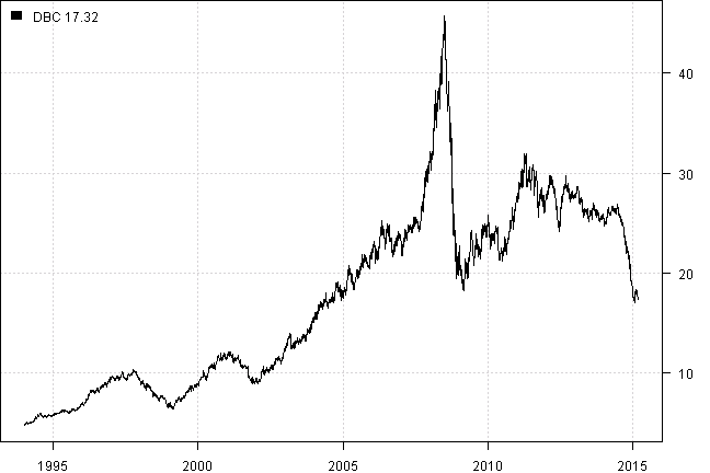
#*****************************************************************
# Helper functions
#*****************************************************************
donchian.channel.breakout.strategy = function(data, lockback.len, long.only=F, use.close=F) {
  if(use.close) {
    high.channel = bt.apply.matrix(data$prices, runMax, lockback.len)
    low.channel = bt.apply.matrix(data$prices, runMin, lockback.len)
   } else {
    phigh = bt.apply(data, Hi)
    plow = bt.apply(data, Lo)

    high.channel = bt.apply.matrix(phigh, runMax, lockback.len)
    low.channel = bt.apply.matrix(plow, runMin, lockback.len)
  }

  data$weight[] = NA
    if(use.close)
      data$weight[] = iif(data$prices == high.channel, 1, iif(data$prices == low.channel, -1, NA))
    else
      data$weight[] = iif(phigh == high.channel, 1, iif(plow == low.channel, iif(long.only,0,-1), NA))
  bt.run.share(data, clean.signal=T, silent=T)
}

percentile.channel.breakout.strategy = function(data, lockback.len, long.only=F) {
  high.channel = bt.apply.matrix(data$prices, runQuantile, lockback.len, probs=0.75)
  low.channel = bt.apply.matrix(data$prices, runQuantile, lockback.len, probs=0.25)

  data$weight[] = NA
    data$weight[] = iif(cross.up(prices, high.channel), 1, iif(cross.dn(prices, low.channel), iif(long.only,0,-1), NA))
  bt.run.share(data, clean.signal=T, silent=T)
}

#*****************************************************************
# Setup
#*****************************************************************
prices = data$prices

models = list()

#*****************************************************************
# Donchian Channel Breakout strategy
#*****************************************************************
models$Donchian55 = donchian.channel.breakout.strategy(data, 55)
models$Donchian55.Long = donchian.channel.breakout.strategy(data, 55, long.only=T)

print('#Transition Map for Donchian Channel Breakout strategy using 55 day lookback:')
#Transition Map for Donchian Channel Breakout strategy using 55 day lookback:
plotbt.transition.map(models$Donchian55$weight)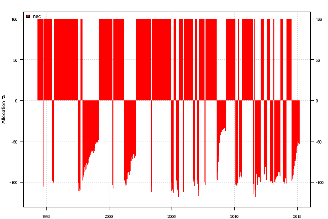
#*****************************************************************
# Percentile Channel Breakout strategy
#*****************************************************************
models$Percentile55 = percentile.channel.breakout.strategy(data, 55)
models$Percentile55.Long = percentile.channel.breakout.strategy(data, 55, long.only=T)

print('#Transition Map for Percentile Channel Breakout strategy using 55 day lookback:')
#Transition Map for Percentile Channel Breakout strategy using 55 day lookback:
plotbt.transition.map(models$Percentile55$weight)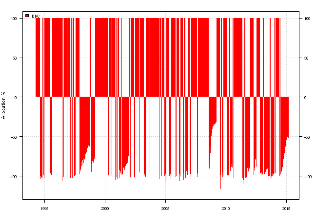
models$Donchian20 = donchian.channel.breakout.strategy(data, 20)
models$Percentile20 = percentile.channel.breakout.strategy(data, 20)

#*****************************************************************
# Report
#strategy.performance.snapshoot(models, T)
plotbt(models, plotX = T, log = 'y', LeftMargin = 3, main = NULL)
	mtext('Cumulative Performance', side = 2, line = 1)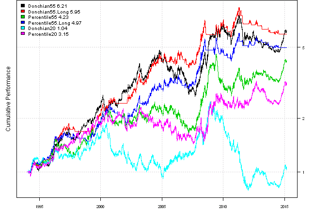
print(plotbt.strategy.sidebyside(models, make.plot=F, return.table=T))| Donchian55 | Donchian55.Long | Percentile55 | Percentile55.Long | Donchian20 | Percentile20 | |
|---|---|---|---|---|---|---|
| Period | Jan1994 - Mar2015 | Jan1994 - Mar2015 | Jan1994 - Mar2015 | Jan1994 - Mar2015 | Jan1994 - Mar2015 | Jan1994 - Mar2015 |
| Cagr | 8.99 | 8.77 | 7.04 | 7.85 | 0.17 | 5.56 |
| Sharpe | 0.63 | 0.72 | 0.51 | 0.68 | 0.09 | 0.42 |
| DVR | 0.53 | 0.66 | 0.42 | 0.63 | 0 | 0.3 |
| Volatility | 15.49 | 12.77 | 15.66 | 12.33 | 16.09 | 16.16 |
| MaxDD | -44.97 | -29.1 | -42.09 | -26.25 | -68.3 | -37.87 |
| AvgDD | -3.13 | -2.8 | -3.88 | -3.05 | -4.75 | -3.55 |
| VaR | -1.54 | -1.29 | -1.57 | -1.25 | -1.64 | -1.63 |
| CVaR | -2.16 | -1.94 | -2.19 | -1.89 | -2.3 | -2.28 |
| Exposure | 98.63 | 63.06 | 98.8 | 59.08 | 99.62 | 99.42 |
Unfortunately we cannot replicate results from original source
I.e. Percentile vs Donchian there is no clear winner in our tests.
Next, let’s examine the A Simple Tactical Asset Allocation Portfolio with Percentile Channels in more details:
#*****************************************************************
# Load historical data
#*****************************************************************
library(SIT)
load.packages('quantmod')

# load saved Proxies Raw Data, data.proxy.raw
# please see http://systematicinvestor.github.io/Data-Proxy/ for more details
load('data/data.proxy.raw.Rdata')

tickers = '
EQ = VTI +VTSMX # (or SPY)
RE = IYR + VGSIX # (or ICF)
CORP.FI = LQD + VWESX
COM = DBC + CRB
CASH = SHY + TB3Y
'

data <- new.env()
getSymbols.extra(tickers, src = 'yahoo', from = '1970-01-01', env = data, raw.data = data.proxy.raw, set.symbolnames = T, auto.assign = T)
for(i in data$symbolnames) data[[i]] = adjustOHLC(data[[i]], use.Adjusted=T)

#print(bt.start.dates(data))
bt.prep(data, align='remove.na', fill.gaps = T)

# Check data
plota.matplot(scale.one(data$prices),main='Asset Perfromance')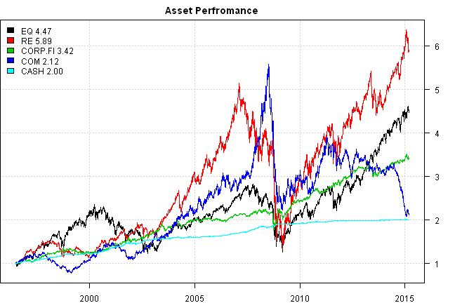
#*****************************************************************
# Setup
#*****************************************************************
data$universe = data$prices > 0
# do not allocate to CASH, or BENCH
data$universe$CASH = NA
prices = data$prices * data$universe
n = ncol(prices)
nperiods = nrow(prices)
frequency = 'months'
# find period ends, can be 'weeks', 'months', 'quarters', 'years'
period.ends = endpoints(prices, frequency)
period.ends = period.ends[period.ends > 0]
models = list()
commission = list(cps = 0.01, fixed = 10.0, percentage = 0.0)
# lag prices by 1 day
#prices = mlag(prices)
#*****************************************************************
# Equal Weight each re-balancing period
#******************************************************************
data$weight[] = NA
data$weight[period.ends,] = ntop(prices[period.ends,], n)
models$ew = bt.run.share(data, clean.signal=F, commission = commission, trade.summary=T, silent=T)
#*****************************************************************
# Risk Parity each re-balancing period
#******************************************************************
ret = diff(log(prices))
hist.vol = sqrt(252) * bt.apply.matrix(ret, runSD, n = 20)
# risk-parity
weight = 1 / hist.vol
rp.weight = weight / rowSums(weight, na.rm=T)
data$weight[] = NA
data$weight[period.ends,] = rp.weight[period.ends,]
models$rp = bt.run.share(data, clean.signal=F, commission = commission, trade.summary=T, silent=T)
#*****************************************************************
# Helper functions
#*****************************************************************
reallocate = function(allocation, data, period.ends, lookback.len,
prefix = '',
min.risk.fns = 'min.var.portfolio',
silent = F
) {
allocation = ifna(allocation, 0)[period.ends,]
# only allocate to selected assets
obj = portfolio.allocation.helper(
data$prices,
period.ends=period.ends,
lookback.len = lookback.len,
universe = allocation > 0,
prefix = prefix,
min.risk.fns = min.risk.fns,
silent = silent
)
# rescale weights to be proportionate allocation
for(i in names(obj$weights)) {
weight = allocation * obj$weights[[i]]
weight = ifna(rowSums(allocation) * weight / rowSums(weight), 0)
weight$CASH = 1 - rowSums(weight)
obj$weights[[i]] = weight
}
create.strategies(obj, data, silent = silent)$models
}
#*****************************************************************
# Strategy:
#
# 1) Use 60,120,180, 252-day percentile channels
# - corresponding to 3,6,9 and 12 months in the momentum literature-
# (4 separate systems) with a .75 long entry and .25 exit threshold with
# long triggered above .75 and holding through until exiting below .25
# (just like in the previous post) - no shorts!!!
#
# 2) If the indicator shows that you should be in cash, hold SHY
#
# 3) Use 20-day historical volatility for risk parity position-sizing
# among active assets (no leverage is used). This is 1/volatility (asset A)
# divided by the sum of 1/volatility for all assets to determine the position size.
#******************************************************************
allocation = 0 * ifna(prices, 0)
for(lockback.len in c(60,120,180, 252)) {
high.channel = bt.apply.matrix(data$prices, runQuantile, lockback.len, probs=0.75)
low.channel = bt.apply.matrix(data$prices, runQuantile, lockback.len, probs=0.25)
signal = iif(cross.up(prices, high.channel), 1, iif(cross.dn(prices, low.channel), 0, NA))
allocation = allocation + ifna( bt.apply.matrix(signal, ifna.prev), 0)
}
# convert to weights, i.e. 4 assets times 4 systems
allocation = allocation / (4 * 4)
# equal-weight
weight = allocation
weight$CASH = 1 - rowSums(weight)
data$weight[] = NA
data$weight[period.ends,] = weight[period.ends,]
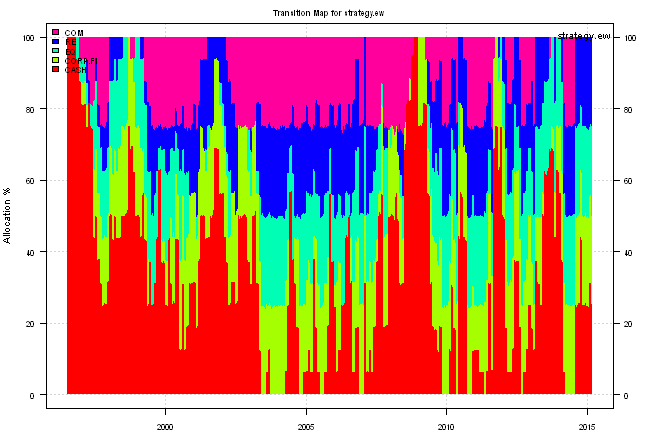
models$strategy.ew = bt.run.share(data, clean.signal=F, commission = commission, trade.summary=T, silent=T)
# risk-parity
weight = allocation * rp.weight
weight = rowSums(allocation, na.rm=T) * weight / rowSums(weight, na.rm=T)
weight$CASH = 1 - rowSums(weight, na.rm=T)
data$weight[] = NA
data$weight[period.ends,] = ifna(weight[period.ends,], 0)
models$strategy.rp = bt.run.share(data, clean.signal=F, commission = commission, trade.summary=T, silent=T)
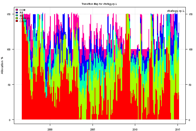
# let's apply leverage
weight1 = ifna(weight, 0)
data$weight[] = NA
data$weight[period.ends,] = target.vol.strategy(models$strategy.rp, weight1,
target=6/100, lookback.len=2*20, max.portfolio.leverage=150/100)[period.ends,]
rs = rowSums(data$weight, na.rm=T)[period.ends]
data$weight$CASH[period.ends] = data$weight$CASH[period.ends] + iif(rs > 1, 0, 1-rs)
models$strategy.rp.L = bt.run.share(data, clean.signal=F, commission = commission, trade.summary=T, silent=T)
#*****************************************************************
# Alternative Way
#*****************************************************************
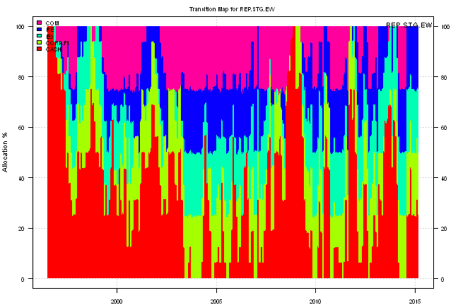
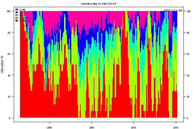
models = c(models,
reallocate(allocation, data, period.ends, 20,
prefix = 'REP.STG.',
min.risk.fns = list(
EW=equal.weight.portfolio,
RP=risk.parity.portfolio()
),
silent = T
)
)Let’s add another benchmark, for comparison we will use the Quantitative Approach To Tactical Asset Allocation Strategy(QATAA) by Mebane T. Faber
#*****************************************************************
#The [Quantitative Approach To Tactical Asset Allocation Strategy(QATAA) by Mebane T. Faber](http://mebfaber.com/timing-model/)
#[SSRN paper](http://papers.ssrn.com/sol3/papers.cfm?abstract_id=962461)
#******************************************************************
# compute 10 month moving average
sma = bt.apply.matrix(prices, SMA, 200)
# go to cash if prices falls below 10 month moving average
go2cash = prices < sma
go2cash = ifna(go2cash, T)
# equal weight target allocation
target.allocation = ntop(prices,n)
# If asset is above it's 10 month moving average it gets allocation
qt.weight = iif(go2cash, 0, target.allocation)
# otherwise, it's weight is allocated to cash
weight = qt.weight
weight$CASH = 1 - rowSums(weight)
data$weight[] = NA
data$weight[period.ends,] = weight[period.ends,]
models$QATAA.EW = bt.run.share(data, clean.signal=F, commission = commission, trade.summary=T, silent=T)
# same, but risk-parity
weight = qt.weight * rp.weight
weight = rowSums(qt.weight, na.rm=T) * weight / rowSums(weight, na.rm=T)
weight$CASH = 1 - rowSums(weight, na.rm=T)
data$weight[] = NA
data$weight[period.ends,] = ifna(weight[period.ends,], 0)
models$QATAA.RP = bt.run.share(data, clean.signal=F, commission = commission, trade.summary=T, silent=T)
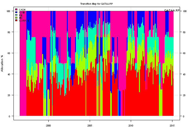
#*****************************************************************
# Alternative Way
#*****************************************************************
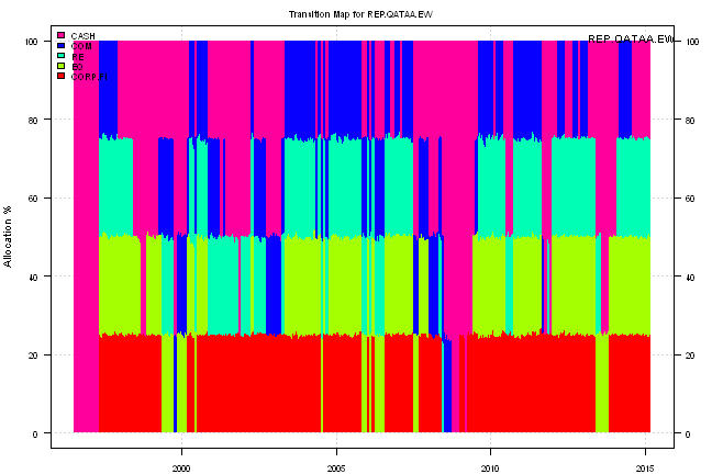
models = c(models,
reallocate(qt.weight, data, period.ends, 20,
prefix = 'REP.QATAA.',
min.risk.fns = list(
EW=equal.weight.portfolio,
RP=risk.parity.portfolio()
),
silent = T
)
)
#*****************************************************************
# Report
#*****************************************************************
#strategy.performance.snapshoot(models, T)
plotbt(models, plotX = T, log = 'y', LeftMargin = 3, main = NULL)
mtext('Cumulative Performance', side = 2, line = 1)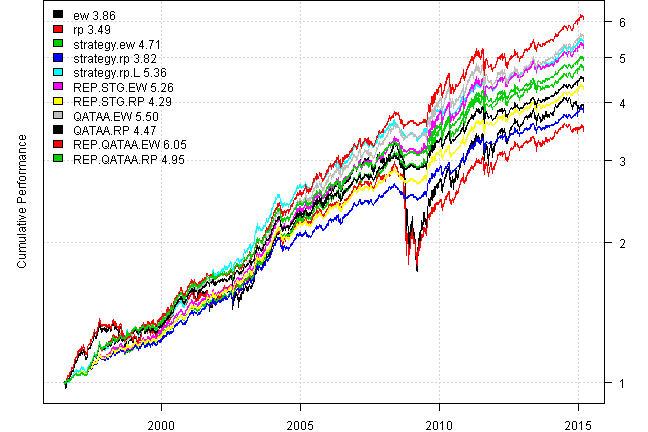
print(plotbt.strategy.sidebyside(models, make.plot=F, return.table=T))| ew | rp | strategy.ew | strategy.rp | strategy.rp.L | REP.STG.EW | REP.STG.RP | QATAA.EW | QATAA.RP | REP.QATAA.EW | REP.QATAA.RP | |
|---|---|---|---|---|---|---|---|---|---|---|---|
| Period | Jun1996 - Mar2015 | Jun1996 - Mar2015 | Jun1996 - Mar2015 | Jun1996 - Mar2015 | Jun1996 - Mar2015 | Jun1996 - Mar2015 | Jun1996 - Mar2015 | Jun1996 - Mar2015 | Jun1996 - Mar2015 | Jun1996 - Mar2015 | Jun1996 - Mar2015 |
| Cagr | 7.48 | 6.91 | 8.64 | 7.43 | 9.39 | 9.28 | 8.09 | 9.54 | 8.33 | 10.1 | 8.92 |
| Sharpe | 0.63 | 0.78 | 1.26 | 1.4 | 1.47 | 1.34 | 1.51 | 1.28 | 1.43 | 1.35 | 1.52 |
| DVR | 0.58 | 0.72 | 1.22 | 1.37 | 1.44 | 1.3 | 1.48 | 1.24 | 1.41 | 1.31 | 1.5 |
| Volatility | 12.76 | 9.17 | 6.81 | 5.25 | 6.28 | 6.82 | 5.26 | 7.36 | 5.72 | 7.37 | 5.73 |
| MaxDD | -47.62 | -40.3 | -11.68 | -8.28 | -10.36 | -11.53 | -7.99 | -12.58 | -8.89 | -12.47 | -8.78 |
| AvgDD | -1.47 | -1.19 | -0.93 | -0.84 | -1.04 | -0.93 | -0.8 | -1.04 | -0.86 | -1.01 | -0.84 |
| VaR | -1.08 | -0.76 | -0.65 | -0.51 | -0.59 | -0.64 | -0.5 | -0.7 | -0.56 | -0.7 | -0.56 |
| CVaR | -1.94 | -1.34 | -1 | -0.76 | -0.89 | -1 | -0.76 | -1.08 | -0.83 | -1.08 | -0.83 |
| Exposure | 99.98 | 99.51 | 99.98 | 99.98 | 99.04 | 99.98 | 99.98 | 99.98 | 99.98 | 99.98 | 99.98 |
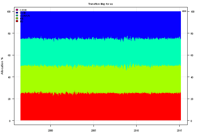
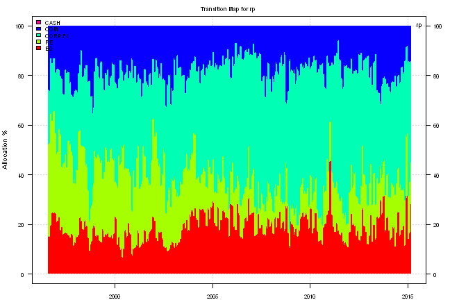
for(m in names(models)) {
  print('#', m)
  plotbt.transition.map(models[[m]]$weight, name=m)
    legend('topright', legend = m, bty = 'n')

  print('Last Trades:')
  print(last.trades(models[m],make.plot=F, return.table=T))

  print('Current Allocation:')
  print(to.percent(last(models[[m]]$weight)))
}
ew
Last Trades:
| ew | weight | entry.date | exit.date | nhold | entry.price | exit.price | return |
|---|---|---|---|---|---|---|---|
| EQ | 25 | 2014-10-31 | 2014-11-28 | 28 | 103.47 | 106.04 | 0.62 |
| RE | 25 | 2014-10-31 | 2014-11-28 | 28 | 74.21 | 76.23 | 0.68 |
| CORP.FI | 25 | 2014-10-31 | 2014-11-28 | 28 | 118.03 | 119.11 | 0.23 |
| COM | 25 | 2014-10-31 | 2014-11-28 | 28 | 22.32 | 20.42 | -2.13 |
| EQ | 25 | 2014-11-28 | 2014-12-31 | 33 | 106.04 | 106.00 | -0.01 |
| RE | 25 | 2014-11-28 | 2014-12-31 | 33 | 76.23 | 76.84 | 0.20 |
| CORP.FI | 25 | 2014-11-28 | 2014-12-31 | 33 | 119.11 | 119.09 | 0.00 |
| COM | 25 | 2014-11-28 | 2014-12-31 | 33 | 20.42 | 18.45 | -2.41 |
| EQ | 25 | 2014-12-31 | 2015-01-30 | 30 | 106.00 | 103.10 | -0.68 |
| RE | 25 | 2014-12-31 | 2015-01-30 | 30 | 76.84 | 81.23 | 1.43 |
| CORP.FI | 25 | 2014-12-31 | 2015-01-30 | 30 | 119.09 | 123.55 | 0.94 |
| COM | 25 | 2014-12-31 | 2015-01-30 | 30 | 18.45 | 17.40 | -1.42 |
| EQ | 25 | 2015-01-30 | 2015-02-27 | 28 | 103.10 | 109.02 | 1.44 |
| RE | 25 | 2015-01-30 | 2015-02-27 | 28 | 81.23 | 79.12 | -0.65 |
| CORP.FI | 25 | 2015-01-30 | 2015-02-27 | 28 | 123.55 | 121.47 | -0.42 |
| COM | 25 | 2015-01-30 | 2015-02-27 | 28 | 17.40 | 18.17 | 1.11 |
| EQ | 25 | 2015-02-27 | 2015-03-11 | 12 | 109.02 | 106.14 | -0.66 |
| RE | 25 | 2015-02-27 | 2015-03-11 | 12 | 79.12 | 76.83 | -0.72 |
| CORP.FI | 25 | 2015-02-27 | 2015-03-11 | 12 | 121.47 | 120.43 | -0.21 |
| COM | 25 | 2015-02-27 | 2015-03-11 | 12 | 18.17 | 17.38 | -1.09 |
Current Allocation:
| EQ | RE | CORP.FI | COM | CASH | |
|---|---|---|---|---|---|
| 2015-03-11 | 25.10% | 24.98% | 25.41% | 24.51% | 0.00% |
rp
Last Trades:
| rp | weight | entry.date | exit.date | nhold | entry.price | exit.price | return |
|---|---|---|---|---|---|---|---|
| EQ | 11.2 | 2014-10-31 | 2014-11-28 | 28 | 103.47 | 106.04 | 0.28 |
| RE | 18.0 | 2014-10-31 | 2014-11-28 | 28 | 74.21 | 76.23 | 0.49 |
| CORP.FI | 56.3 | 2014-10-31 | 2014-11-28 | 28 | 118.03 | 119.11 | 0.51 |
| COM | 14.5 | 2014-10-31 | 2014-11-28 | 28 | 22.32 | 20.42 | -1.24 |
| EQ | 31.1 | 2014-11-28 | 2014-12-31 | 33 | 106.04 | 106.00 | -0.01 |
| RE | 24.6 | 2014-11-28 | 2014-12-31 | 33 | 76.23 | 76.84 | 0.20 |
| CORP.FI | 35.4 | 2014-11-28 | 2014-12-31 | 33 | 119.11 | 119.09 | -0.01 |
| COM | 8.9 | 2014-11-28 | 2014-12-31 | 33 | 20.42 | 18.45 | -0.86 |
| EQ | 14.3 | 2014-12-31 | 2015-01-30 | 30 | 106.00 | 103.10 | -0.39 |
| RE | 16.3 | 2014-12-31 | 2015-01-30 | 30 | 76.84 | 81.23 | 0.93 |
| CORP.FI | 53.9 | 2014-12-31 | 2015-01-30 | 30 | 119.09 | 123.55 | 2.02 |
| COM | 15.5 | 2014-12-31 | 2015-01-30 | 30 | 18.45 | 17.40 | -0.88 |
| EQ | 15.9 | 2015-01-30 | 2015-02-27 | 28 | 103.10 | 109.02 | 0.91 |
| RE | 20.5 | 2015-01-30 | 2015-02-27 | 28 | 81.23 | 79.12 | -0.53 |
| CORP.FI | 49.3 | 2015-01-30 | 2015-02-27 | 28 | 123.55 | 121.47 | -0.83 |
| COM | 14.3 | 2015-01-30 | 2015-02-27 | 28 | 17.40 | 18.17 | 0.63 |
| EQ | 27.7 | 2015-02-27 | 2015-03-11 | 12 | 109.02 | 106.14 | -0.73 |
| RE | 17.0 | 2015-02-27 | 2015-03-11 | 12 | 79.12 | 76.83 | -0.49 |
| CORP.FI | 40.8 | 2015-02-27 | 2015-03-11 | 12 | 121.47 | 120.43 | -0.35 |
| COM | 14.5 | 2015-02-27 | 2015-03-11 | 12 | 18.17 | 17.38 | -0.63 |
Current Allocation:
| EQ | RE | CORP.FI | COM | CASH | |
|---|---|---|---|---|---|
| 2015-03-11 | 27.70% | 16.89% | 41.29% | 14.12% | 0.00% |
strategy.ew
Last Trades:
| strategy.ew | weight | entry.date | exit.date | nhold | entry.price | exit.price | return |
|---|---|---|---|---|---|---|---|
| EQ | 25.0 | 2014-10-31 | 2014-11-28 | 28 | 103.47 | 106.04 | 0.62 |
| RE | 25.0 | 2014-10-31 | 2014-11-28 | 28 | 74.21 | 76.23 | 0.68 |
| CORP.FI | 25.0 | 2014-10-31 | 2014-11-28 | 28 | 118.03 | 119.11 | 0.23 |
| CASH | 25.0 | 2014-10-31 | 2014-11-28 | 28 | 84.61 | 84.70 | 0.03 |
| EQ | 25.0 | 2014-11-28 | 2014-12-31 | 33 | 106.04 | 106.00 | -0.01 |
| RE | 25.0 | 2014-11-28 | 2014-12-31 | 33 | 76.23 | 76.84 | 0.20 |
| CORP.FI | 25.0 | 2014-11-28 | 2014-12-31 | 33 | 119.11 | 119.09 | 0.00 |
| CASH | 25.0 | 2014-11-28 | 2014-12-31 | 33 | 84.70 | 84.42 | -0.08 |
| EQ | 25.0 | 2014-12-31 | 2015-01-30 | 30 | 106.00 | 103.10 | -0.68 |
| RE | 25.0 | 2014-12-31 | 2015-01-30 | 30 | 76.84 | 81.23 | 1.43 |
| CORP.FI | 25.0 | 2014-12-31 | 2015-01-30 | 30 | 119.09 | 123.55 | 0.94 |
| CASH | 25.0 | 2014-12-31 | 2015-01-30 | 30 | 84.42 | 84.95 | 0.16 |
| EQ | 18.8 | 2015-01-30 | 2015-02-27 | 28 | 103.10 | 109.02 | 1.08 |
| RE | 25.0 | 2015-01-30 | 2015-02-27 | 28 | 81.23 | 79.12 | -0.65 |
| CORP.FI | 25.0 | 2015-01-30 | 2015-02-27 | 28 | 123.55 | 121.47 | -0.42 |
| CASH | 31.2 | 2015-01-30 | 2015-02-27 | 28 | 84.95 | 84.67 | -0.10 |
| EQ | 25.0 | 2015-02-27 | 2015-03-11 | 12 | 109.02 | 106.14 | -0.66 |
| RE | 25.0 | 2015-02-27 | 2015-03-11 | 12 | 79.12 | 76.83 | -0.72 |
| CORP.FI | 25.0 | 2015-02-27 | 2015-03-11 | 12 | 121.47 | 120.43 | -0.21 |
| CASH | 25.0 | 2015-02-27 | 2015-03-11 | 12 | 84.67 | 84.60 | -0.02 |
Current Allocation:
| EQ | RE | CORP.FI | COM | CASH | |
|---|---|---|---|---|---|
| 2015-03-11 | 24.79% | 24.68% | 25.10% | 0.00% | 25.43% |
strategy.rp

Last Trades:
| strategy.rp | weight | entry.date | exit.date | nhold | entry.price | exit.price | return |
|---|---|---|---|---|---|---|---|
| EQ | 9.8 | 2014-10-31 | 2014-11-28 | 28 | 103.47 | 106.04 | 0.24 |
| RE | 15.8 | 2014-10-31 | 2014-11-28 | 28 | 74.21 | 76.23 | 0.43 |
| CORP.FI | 49.4 | 2014-10-31 | 2014-11-28 | 28 | 118.03 | 119.11 | 0.45 |
| CASH | 25.0 | 2014-10-31 | 2014-11-28 | 28 | 84.61 | 84.70 | 0.03 |
| EQ | 25.6 | 2014-11-28 | 2014-12-31 | 33 | 106.04 | 106.00 | -0.01 |
| RE | 20.2 | 2014-11-28 | 2014-12-31 | 33 | 76.23 | 76.84 | 0.16 |
| CORP.FI | 29.2 | 2014-11-28 | 2014-12-31 | 33 | 119.11 | 119.09 | 0.00 |
| CASH | 25.0 | 2014-11-28 | 2014-12-31 | 33 | 84.70 | 84.42 | -0.08 |
| EQ | 12.7 | 2014-12-31 | 2015-01-30 | 30 | 106.00 | 103.10 | -0.35 |
| RE | 14.5 | 2014-12-31 | 2015-01-30 | 30 | 76.84 | 81.23 | 0.83 |
| CORP.FI | 47.8 | 2014-12-31 | 2015-01-30 | 30 | 119.09 | 123.55 | 1.79 |
| CASH | 25.0 | 2014-12-31 | 2015-01-30 | 30 | 84.42 | 84.95 | 0.16 |
| EQ | 10.0 | 2015-01-30 | 2015-02-27 | 28 | 103.10 | 109.02 | 0.58 |
| RE | 17.2 | 2015-01-30 | 2015-02-27 | 28 | 81.23 | 79.12 | -0.45 |
| CORP.FI | 41.5 | 2015-01-30 | 2015-02-27 | 28 | 123.55 | 121.47 | -0.70 |
| CASH | 31.2 | 2015-01-30 | 2015-02-27 | 28 | 84.95 | 84.67 | -0.10 |
| EQ | 24.3 | 2015-02-27 | 2015-03-11 | 12 | 109.02 | 106.14 | -0.64 |
| RE | 14.9 | 2015-02-27 | 2015-03-11 | 12 | 79.12 | 76.83 | -0.43 |
| CORP.FI | 35.8 | 2015-02-27 | 2015-03-11 | 12 | 121.47 | 120.43 | -0.31 |
| CASH | 25.0 | 2015-02-27 | 2015-03-11 | 12 | 84.67 | 84.60 | -0.02 |
Current Allocation:
| EQ | RE | CORP.FI | COM | CASH | |
|---|---|---|---|---|---|
| 2015-03-11 | 24.07% | 14.67% | 35.88% | 0.00% | 25.38% |
strategy.rp.L
Last Trades:
| strategy.rp.L | weight | entry.date | exit.date | nhold | entry.price | exit.price | return |
|---|---|---|---|---|---|---|---|
| EQ | 14.7 | 2014-10-31 | 2014-11-28 | 28 | 103.47 | 106.04 | 0.37 |
| RE | 23.7 | 2014-10-31 | 2014-11-28 | 28 | 74.21 | 76.23 | 0.64 |
| CORP.FI | 74.1 | 2014-10-31 | 2014-11-28 | 28 | 118.03 | 119.11 | 0.68 |
| CASH | 37.5 | 2014-10-31 | 2014-11-28 | 28 | 84.61 | 84.70 | 0.04 |
| EQ | 38.4 | 2014-11-28 | 2014-12-31 | 33 | 106.04 | 106.00 | -0.01 |
| RE | 30.4 | 2014-11-28 | 2014-12-31 | 33 | 76.23 | 76.84 | 0.24 |
| CORP.FI | 43.8 | 2014-11-28 | 2014-12-31 | 33 | 119.11 | 119.09 | -0.01 |
| CASH | 37.5 | 2014-11-28 | 2014-12-31 | 33 | 84.70 | 84.42 | -0.12 |
| EQ | 14.9 | 2014-12-31 | 2015-01-30 | 30 | 106.00 | 103.10 | -0.41 |
| RE | 16.9 | 2014-12-31 | 2015-01-30 | 30 | 76.84 | 81.23 | 0.97 |
| CORP.FI | 56.0 | 2014-12-31 | 2015-01-30 | 30 | 119.09 | 123.55 | 2.10 |
| CASH | 29.3 | 2014-12-31 | 2015-01-30 | 30 | 84.42 | 84.95 | 0.18 |
| EQ | 12.3 | 2015-01-30 | 2015-02-27 | 28 | 103.10 | 109.02 | 0.71 |
| RE | 21.2 | 2015-01-30 | 2015-02-27 | 28 | 81.23 | 79.12 | -0.55 |
| CORP.FI | 51.0 | 2015-01-30 | 2015-02-27 | 28 | 123.55 | 121.47 | -0.86 |
| CASH | 38.4 | 2015-01-30 | 2015-02-27 | 28 | 84.95 | 84.67 | -0.13 |
| EQ | 33.5 | 2015-02-27 | 2015-03-11 | 12 | 109.02 | 106.14 | -0.88 |
| RE | 20.5 | 2015-02-27 | 2015-03-11 | 12 | 79.12 | 76.83 | -0.59 |
| CORP.FI | 49.3 | 2015-02-27 | 2015-03-11 | 12 | 121.47 | 120.43 | -0.42 |
| CASH | 34.4 | 2015-02-27 | 2015-03-11 | 12 | 84.67 | 84.60 | -0.03 |
Current Allocation:
| EQ | RE | CORP.FI | COM | CASH | |
|---|---|---|---|---|---|
| 2015-03-11 | 33.36% | 20.34% | 49.73% | 0.00% | 35.18% |
REP.STG.EW
Last Trades:
Current Allocation:
| EQ | RE | CORP.FI | COM | CASH | |
|---|---|---|---|---|---|
| 2015-03-11 | 24.79% | 24.68% | 25.10% | 0.00% | 25.43% |
REP.STG.RP
Last Trades:
Current Allocation:
| EQ | RE | CORP.FI | COM | CASH | |
|---|---|---|---|---|---|
| 2015-03-11 | 23.99% | 14.75% | 35.88% | 0.00% | 25.38% |
QATAA.EW

Last Trades:
| QATAA.EW | weight | entry.date | exit.date | nhold | entry.price | exit.price | return |
|---|---|---|---|---|---|---|---|
| EQ | 25 | 2014-10-31 | 2014-11-28 | 28 | 103.47 | 106.04 | 0.62 |
| RE | 25 | 2014-10-31 | 2014-11-28 | 28 | 74.21 | 76.23 | 0.68 |
| CORP.FI | 25 | 2014-10-31 | 2014-11-28 | 28 | 118.03 | 119.11 | 0.23 |
| CASH | 25 | 2014-10-31 | 2014-11-28 | 28 | 84.61 | 84.70 | 0.03 |
| EQ | 25 | 2014-11-28 | 2014-12-31 | 33 | 106.04 | 106.00 | -0.01 |
| RE | 25 | 2014-11-28 | 2014-12-31 | 33 | 76.23 | 76.84 | 0.20 |
| CORP.FI | 25 | 2014-11-28 | 2014-12-31 | 33 | 119.11 | 119.09 | 0.00 |
| CASH | 25 | 2014-11-28 | 2014-12-31 | 33 | 84.70 | 84.42 | -0.08 |
| EQ | 25 | 2014-12-31 | 2015-01-30 | 30 | 106.00 | 103.10 | -0.68 |
| RE | 25 | 2014-12-31 | 2015-01-30 | 30 | 76.84 | 81.23 | 1.43 |
| CORP.FI | 25 | 2014-12-31 | 2015-01-30 | 30 | 119.09 | 123.55 | 0.94 |
| CASH | 25 | 2014-12-31 | 2015-01-30 | 30 | 84.42 | 84.95 | 0.16 |
| EQ | 25 | 2015-01-30 | 2015-02-27 | 28 | 103.10 | 109.02 | 1.44 |
| RE | 25 | 2015-01-30 | 2015-02-27 | 28 | 81.23 | 79.12 | -0.65 |
| CORP.FI | 25 | 2015-01-30 | 2015-02-27 | 28 | 123.55 | 121.47 | -0.42 |
| CASH | 25 | 2015-01-30 | 2015-02-27 | 28 | 84.95 | 84.67 | -0.08 |
| EQ | 25 | 2015-02-27 | 2015-03-11 | 12 | 109.02 | 106.14 | -0.66 |
| RE | 25 | 2015-02-27 | 2015-03-11 | 12 | 79.12 | 76.83 | -0.72 |
| CORP.FI | 25 | 2015-02-27 | 2015-03-11 | 12 | 121.47 | 120.43 | -0.21 |
| CASH | 25 | 2015-02-27 | 2015-03-11 | 12 | 84.67 | 84.60 | -0.02 |
Current Allocation:
| EQ | RE | CORP.FI | COM | CASH | |
|---|---|---|---|---|---|
| 2015-03-11 | 24.79% | 24.68% | 25.10% | 0.00% | 25.43% |
QATAA.RP
Last Trades:
| QATAA.RP | weight | entry.date | exit.date | nhold | entry.price | exit.price | return |
|---|---|---|---|---|---|---|---|
| EQ | 9.8 | 2014-10-31 | 2014-11-28 | 28 | 103.47 | 106.04 | 0.24 |
| RE | 15.8 | 2014-10-31 | 2014-11-28 | 28 | 74.21 | 76.23 | 0.43 |
| CORP.FI | 49.4 | 2014-10-31 | 2014-11-28 | 28 | 118.03 | 119.11 | 0.45 |
| CASH | 25.0 | 2014-10-31 | 2014-11-28 | 28 | 84.61 | 84.70 | 0.03 |
| EQ | 25.6 | 2014-11-28 | 2014-12-31 | 33 | 106.04 | 106.00 | -0.01 |
| RE | 20.2 | 2014-11-28 | 2014-12-31 | 33 | 76.23 | 76.84 | 0.16 |
| CORP.FI | 29.2 | 2014-11-28 | 2014-12-31 | 33 | 119.11 | 119.09 | 0.00 |
| CASH | 25.0 | 2014-11-28 | 2014-12-31 | 33 | 84.70 | 84.42 | -0.08 |
| EQ | 12.7 | 2014-12-31 | 2015-01-30 | 30 | 106.00 | 103.10 | -0.35 |
| RE | 14.5 | 2014-12-31 | 2015-01-30 | 30 | 76.84 | 81.23 | 0.83 |
| CORP.FI | 47.8 | 2014-12-31 | 2015-01-30 | 30 | 119.09 | 123.55 | 1.79 |
| CASH | 25.0 | 2014-12-31 | 2015-01-30 | 30 | 84.42 | 84.95 | 0.16 |
| EQ | 13.9 | 2015-01-30 | 2015-02-27 | 28 | 103.10 | 109.02 | 0.80 |
| RE | 17.9 | 2015-01-30 | 2015-02-27 | 28 | 81.23 | 79.12 | -0.47 |
| CORP.FI | 43.2 | 2015-01-30 | 2015-02-27 | 28 | 123.55 | 121.47 | -0.73 |
| CASH | 25.0 | 2015-01-30 | 2015-02-27 | 28 | 84.95 | 84.67 | -0.08 |
| EQ | 24.3 | 2015-02-27 | 2015-03-11 | 12 | 109.02 | 106.14 | -0.64 |
| RE | 14.9 | 2015-02-27 | 2015-03-11 | 12 | 79.12 | 76.83 | -0.43 |
| CORP.FI | 35.8 | 2015-02-27 | 2015-03-11 | 12 | 121.47 | 120.43 | -0.31 |
| CASH | 25.0 | 2015-02-27 | 2015-03-11 | 12 | 84.67 | 84.60 | -0.02 |
Current Allocation:
| EQ | RE | CORP.FI | COM | CASH | |
|---|---|---|---|---|---|
| 2015-03-11 | 24.07% | 14.67% | 35.88% | 0.00% | 25.38% |
REP.QATAA.EW
Last Trades:
Current Allocation:
| EQ | RE | CORP.FI | COM | CASH | |
|---|---|---|---|---|---|
| 2015-03-11 | 24.79% | 24.68% | 25.10% | 0.00% | 25.43% |
REP.QATAA.RP

Last Trades:
Current Allocation:
| EQ | RE | CORP.FI | COM | CASH | |
|---|---|---|---|---|---|
| 2015-03-11 | 23.99% | 14.75% | 35.88% | 0.00% | 25.38% |
Unfortunately we cannot match the numbers from original source
But overall, this concept is a very robust allocation framework.
ToDo: take the posts about Permanent Portfolio and apply here systematicinvestor.wordpress.com/?s=Permanent+Portfolio
(this report was produced on: 2015-03-12)