Back-testing Trades
21 Jan 2015To install Systematic Investor Toolbox (SIT) please visit About page.
Once in a while I get questions about how to make an equity curve given historical signal(s) / trade(s).
Let’s take for example the historical signals from MARKET TIMING with DECISION MOOSE and create equity curve for this strategy.
#*****************************************************************
# Load signals from http://www.decisionmoose.com/Moosistory.html
#*****************************************************************
library(SIT)
load.packages('quantmod')


filename = 'data/decisionmoose.Rdata'
if(!file.exists(filename)) {
	url = 'http://www.decisionmoose.com/Moosistory.html'
	txt = join(readLines(url))

	# extract transaction history
	temp = extract.table.from.webpage(txt, 'Transaction History', has.header = F)
		temp = trim(temp[-1,2:5])
 	colnames(temp) = spl('id,date,name,equity')

 id = as.numeric(temp[,'id'])
 	index = ifna(id > 0,F)
 temp = temp[index,]

 temp[,'equity'] = gsub('\\.','',gsub(',','',gsub('\\$','',temp[,'equity'])))
 info = data.frame(stringsAsFactors = F,
 id = as.numeric(temp[,'id']),
 equity = as.numeric(temp[,'equity']),
 date = as.Date(temp[,'date'],'%m.%d.%Y'),
 tickers = toupper(trim(gsub('\\)','', sapply(temp[,'name'], spl, '\\('))))[2,]
 )
 info = info[!is.na(info$date),]
save(info, file=filename)
}

load(file=filename)


#plota(make.xts(info$equity, info$date), type='l')

#*****************************************************************
# Load historical data
#*****************************************************************
tickers = unique(info$tickers)

# load saved Proxies Raw Data, data.proxy.raw
load('data/data.proxy.raw.Rdata')

# define Cash (3moT) 3MOT = BIL+TB3M
tickers = gsub('3MOT','3MOT=BIL+TB3M', tickers)

#US:SAF Scudder New Asia Fund (SAF), Merged into DWS Emerging Markets Equity Fund
#https://www.backrecord.com/topic/us-saf
tickers = gsub('SAF','SAF=SEKCX', tickers)


# add dummy stock, to keep dates of trades, if they do not line up with data
dummy = make.stock.xts(make.xts(info$equity, info$date))

data <- new.env()
getSymbols.extra(tickers, src = 'yahoo', from = '1970-01-01', env = data, raw.data = data.proxy.raw, auto.assign = T)

	# optionally investigate splits not captured by Adjusted
	#data.clean(data, min.ratio=3)

  for(i in ls(data)) data[[i]] = adjustOHLC(data[[i]], use.Adjusted=T)

  #print(bt.start.dates(data))

  data$dummy = dummy

bt.prep(data, align='keep.all', dates='2000::',fill.gaps = T)

bt.prep.remove.symbols(data, 'dummy')

#plota.matplot(scale.one(data$prices),main='Asset Perfromance')

#*****************************************************************
# Setup
#*****************************************************************
prices = data$prices

models = list()

#*****************************************************************
# Code Strategies, SPY - Buy & Hold
#*****************************************************************
data$weight[] = NA
	data$weight$SPY = 1
models$SPY = bt.run.share(data, clean.signal=T, silent=T)

#*****************************************************************
# Create weights
#*****************************************************************
weight = NA * prices

for(t in 1:nrow(info)) {
	weight[info$date[t],] = 0
 weight[info$date[t], info$ticker[t]] = 1
}

data$weight[] = 	weight
models$decisionmoose = bt.run.share(data, clean.signal=F, trade.summary=T, silent=T)#, do.lag = 2)


#*****************************************************************
# Create Report
#******************************************************************
plota.matplot(scale.one(data$prices),main='Asset Perfromance')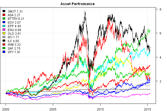
#strategy.performance.snapshoot(models, title = 'decisionmoose', data = data)
plotbt(models, plotX = T, log = 'y', LeftMargin = 3, main = NULL)
	mtext('Cumulative Performance', side = 2, line = 1)
print(plotbt.strategy.sidebyside(models, make.plot=F, return.table=T))| SPY | decisionmoose | |
|---|---|---|
| Period | Jan2000 - Apr2015 | Jan2000 - Apr2015 |
| Cagr | 4.33 | 18.31 |
| Sharpe | 0.31 | 0.91 |
| DVR | 0.16 | 0.89 |
| Volatility | 20.16 | 20.29 |
| MaxDD | -55.19 | -24.43 |
| AvgDD | -2.55 | -4.28 |
| VaR | -1.98 | -2.01 |
| CVaR | -3 | -3 |
| Exposure | 99.97 | 97.68 |
m = 'decisionmoose'
plotbt.transition.map(models[[m]]$weight, name=m)
		legend('topright', legend = m, bty = 'n')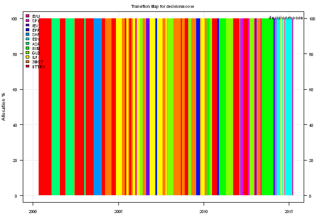
print(last.trades(models$decisionmoose, smain='decisionmoose',make.plot=F, return.table=T))| decisionmoose | weight | entry.date | exit.date | nhold | entry.price | exit.price | return |
|---|---|---|---|---|---|---|---|
| IWM | 100 | 2012-02-10 | 2012-03-02 | 21 | 77.53 | 76.56 | -1.25 |
| SPY | 100 | 2012-03-02 | 2012-05-04 | 63 | 128.57 | 128.85 | 0.22 |
| BTTRX | 100 | 2012-05-04 | 2012-08-10 | 98 | 73.19 | 77.24 | 5.53 |
| SPY | 100 | 2012-08-10 | 2012-09-21 | 42 | 133.14 | 138.64 | 4.13 |
| GLD | 100 | 2012-09-21 | 2012-12-14 | 84 | 171.96 | 164.13 | -4.55 |
| 3MOT | 100 | 2012-12-14 | 2013-01-04 | 21 | 45.81 | 45.82 | 0.02 |
| IEV | 100 | 2013-01-04 | 2013-02-08 | 35 | 37.26 | 38.00 | 1.99 |
| 3MOT | 100 | 2013-02-08 | 2013-05-10 | 91 | 45.81 | 45.80 | -0.02 |
| EWJ | 100 | 2013-05-10 | 2013-05-31 | 21 | 11.47 | 10.58 | -7.76 |
| IWM | 100 | 2013-05-31 | 2014-02-07 | 252 | 95.50 | 109.33 | 14.48 |
| IEV | 100 | 2014-02-07 | 2014-03-07 | 28 | 44.94 | 46.85 | 4.25 |
| IWM | 100 | 2014-03-07 | 2014-04-04 | 28 | 118.17 | 113.32 | -4.10 |
| SPY | 100 | 2014-04-04 | 2014-04-11 | 7 | 182.82 | 178.02 | -2.63 |
| EDV | 100 | 2014-04-11 | 2014-07-03 | 83 | 98.98 | 99.94 | 0.96 |
| ILF | 100 | 2014-07-03 | 2014-08-22 | 50 | 38.17 | 40.24 | 5.42 |
| EDV | 100 | 2014-08-22 | 2014-09-05 | 14 | 109.30 | 108.16 | -1.05 |
| ILF | 100 | 2014-09-05 | 2014-09-26 | 21 | 42.33 | 38.20 | -9.76 |
| SPY | 100 | 2014-09-26 | 2014-10-10 | 14 | 195.94 | 188.65 | -3.72 |
| EDV | 100 | 2014-10-10 | 2015-03-13 | 154 | 114.15 | 124.09 | 8.71 |
| EWJ | 100 | 2015-03-13 | 2015-04-10 | 28 | 12.48 | 12.94 | 3.69 |
(this report was produced on: 2015-04-11)