Back-test Reality Check

19 Oct 2015

To install Systematic Investor Toolbox (SIT) please visit About page.

The purpose of a back-test is to show a realistic historical picture of strategy performance. One might use back-test results and corresponding statistics to judge whether a strategy is suitable one. Hence, it is best to structure a back-test to be as realistic as possible in order to avoid unpleasant surprises and have solid foundation for selecting a suitable strategy.

First strategy outline: the strategy is the strategic equal weight allocation across following 5 stocks: MMM, AA, CAT, KO, HPQ. I selected these stocks from Dow Jones Industrial Average. The allocation is updated monthly and back-test starts on Jan 1st, 1970 with $100,000 initial capital.

Let’s start with the most simple back-test setup and incrementally add features to make it more realistic.

The most simple setup is to multiply weights vector by daily returns, based on adjusted prices, to compute daily returns for the strategy. Please see below the equity line for the strategy (r.ew)

#*****************************************************************
# Load historical data
#*****************************************************************
library(SIT)
load.packages('quantmod')

tickers = 'MMM, AA, CAT, KO, HPQ'

data = env()
getSymbols.extra(tickers, src = 'yahoo', from = '1970-01-01', env = data, set.symbolnames = T, auto.assign = T)
	# copy unadjusted prices
	data.raw = env(data)

	# adjusted prices
	for(i in data$symbolnames) data[[i]] = adjustOHLC(data[[i]], use.Adjusted=T)
bt.prep(data, align='remove.na', fill.gaps = T)

#*****************************************************************
# Setup
#*****************************************************************
prices = data$prices
	n = ncol(prices)
	nperiods = nrow(prices)

period.ends = date.ends(prices,'months')
	  
models = list()
	
commission = list(cps = 0.01, fixed = 10.0, percentage = 0.0)
	
weights = rep.row(rep(1/n, n), len(period.ends))
	
#*****************************************************************
# r.ew
#******************************************************************
data$weight[] = NA
	data$weight[period.ends,] = weights
models$r.ew = bt.run(data, silent=T, trade.summary=T)

#*****************************************************************
# Create Report
#****************************************************************** 
print('#Dividend and Split Adjusted Asset Performance')

#Dividend and Split Adjusted Asset Performance

plota.matplot(scale.one(data$prices),main='Asset Performance')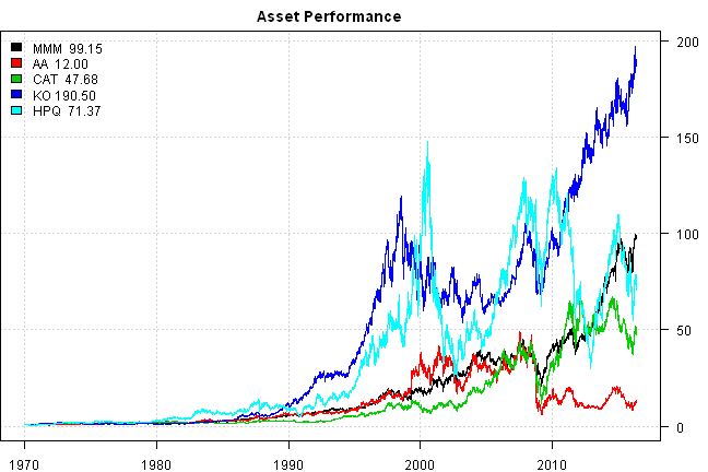

plot of chunk plot-2

plotbt(models, plotX = T, log = 'y', LeftMargin = 3, main = NULL)	    	
	mtext('Cumulative Performance', side = 2, line = 1)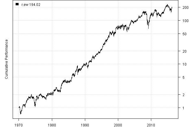

plot of chunk plot-2

print(plotbt.strategy.sidebyside(models, make.plot=F, return.table=T,perfromance.fn = engineering.returns.kpi))

	r.ew
Period	Jan1970 - May2016
Cagr	12.03
Sharpe	0.65
DVR	0.52
R2	0.8
Volatility	20.97
MaxDD	-60.67
Exposure	99.82
Win.Percent	100
Avg.Trade	1765.79
Profit.Factor	NaN
Num.Trades	5

There is a problem with above approach, it assumes that weights stay constant through out the month, or alternatively that we re-balance strategy daily to the target allocation. However, in reality, we invest at the end of the month and update allocations at the end of the next month. The proper solution is to compute share allocation at the end of the month and update shares at the end of the next month (s.ew)

#*****************************************************************
# s.ew
#******************************************************************
data$weight[] = NA
	data$weight[period.ends,] = weights
models$s.ew = bt.run.share.ex(data, clean.signal=F, silent=T, trade.summary=T)

#*****************************************************************
# Create Report
#****************************************************************** 
plotbt(models, plotX = T, log = 'y', LeftMargin = 3, main = NULL)	    	
	mtext('Cumulative Performance', side = 2, line = 1)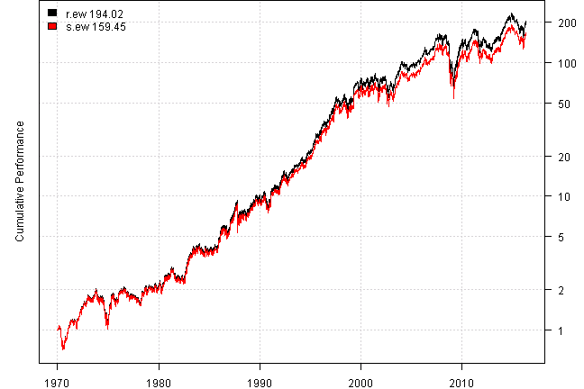

plot of chunk plot-3

print(plotbt.strategy.sidebyside(models, make.plot=F, return.table=T,perfromance.fn = engineering.returns.kpi))

	r.ew	s.ew
Period	Jan1970 - May2016	Jan1970 - May2016
Cagr	12.03	11.56
Sharpe	0.65	0.63
DVR	0.52	0.51
R2	0.8	0.81
Volatility	20.97	20.89
MaxDD	-60.67	-60.88
Exposure	99.82	99.82
Win.Percent	100	55.62
Avg.Trade	1765.79	0.21
Profit.Factor	NaN	1.4
Num.Trades	5	2785

One of the missing features of above approach is commissions. In reality, every time we make a transaction, brokerage charge commissions. Let’s add following commission structure: $10 fixed per transaction, plus 1c per share (s.ew.com)

#*****************************************************************
# s.ew.com
#******************************************************************
data$weight[] = NA
	data$weight[period.ends,] = weights
models$s.ew.com = bt.run.share.ex(data, clean.signal=F, silent=T, commission=commission, trade.summary=T)

#*****************************************************************
# Create Report
#****************************************************************** 
plotbt(models, plotX = T, log = 'y', LeftMargin = 3, main = NULL)	    	
	mtext('Cumulative Performance', side = 2, line = 1)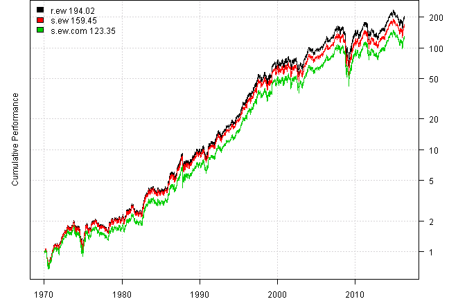

plot of chunk plot-4

print(plotbt.strategy.sidebyside(models, make.plot=F, return.table=T,perfromance.fn = engineering.returns.kpi))

	r.ew	s.ew	s.ew.com
Period	Jan1970 - May2016	Jan1970 - May2016	Jan1970 - May2016
Cagr	12.03	11.56	10.94
Sharpe	0.65	0.63	0.6
DVR	0.52	0.51	0.49
R2	0.8	0.81	0.81
Volatility	20.97	20.89	20.89
MaxDD	-60.67	-60.88	-60.9
Exposure	99.82	99.82	99.82
Win.Percent	100	55.62	55.62
Avg.Trade	1765.79	0.21	0.21
Profit.Factor	NaN	1.4	1.4
Num.Trades	5	2785	2785

Another missing feature of above approach is round lot share allocation. In reality, we don’t acquire fractional shares, most of the time we buy shares in round lots. Let’s add 100 shares round lot requirement (s.ew.com.lot)

#*****************************************************************
# s.ew.com.lot
#******************************************************************
data$weight[] = NA
	data$weight[period.ends,] = weights
models$s.ew.com.lot = bt.run.share.ex(data, clean.signal=F, silent=T, commission=commission, trade.summary=T,
	lot.size=100
)

#*****************************************************************
# Create Report
#****************************************************************** 
plotbt(models, plotX = T, log = 'y', LeftMargin = 3, main = NULL)	    	
	mtext('Cumulative Performance', side = 2, line = 1)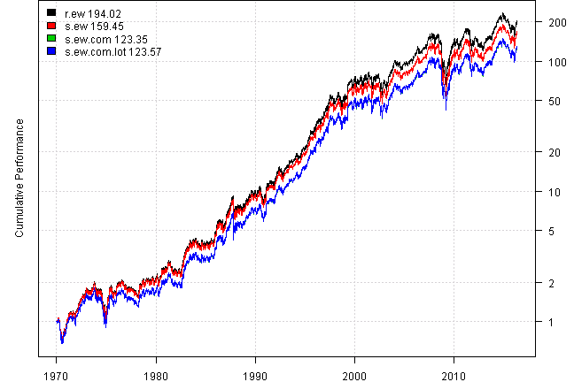

plot of chunk plot-5

print(plotbt.strategy.sidebyside(models, make.plot=F, return.table=T,perfromance.fn = engineering.returns.kpi))

	r.ew	s.ew	s.ew.com	s.ew.com.lot
Period	Jan1970 - May2016	Jan1970 - May2016	Jan1970 - May2016	Jan1970 - May2016
Cagr	12.03	11.56	10.94	10.95
Sharpe	0.65	0.63	0.6	0.6
DVR	0.52	0.51	0.49	0.49
R2	0.8	0.81	0.81	0.81
Volatility	20.97	20.89	20.89	20.88
MaxDD	-60.67	-60.88	-60.9	-60.89
Exposure	99.82	99.82	99.82	99.82
Win.Percent	100	55.62	55.62	55.25
Avg.Trade	1765.79	0.21	0.21	0.22
Profit.Factor	NaN	1.4	1.4	1.41
Num.Trades	5	2785	2785	2726

Another missing feature of above approach is turnover control. In reality, we don’t blindly re-balance to new allocation, but instead evaluate the cost of re-balance and tracking error, and only re-balance when needed. Let’s re-balance only if total absolute discrepancy between current allocation and target allocation is greater than 5% (s.ew.com.lot.turnover)

#*****************************************************************
# s.ew.com.lot.turnover
#******************************************************************
data$weight[] = NA
	data$weight[period.ends,] = weights
models$s.ew.com.lot.turnover = bt.run.share.ex(data, clean.signal=F, silent=T, commission=commission, trade.summary=T,
	lot.size=100,
	control = list(round.lot = list(select = 'minimum.turnover', diff.target = 5/100))
)

#*****************************************************************
# Create Report
#****************************************************************** 
plotbt(models, plotX = T, log = 'y', LeftMargin = 3, main = NULL)	    	
	mtext('Cumulative Performance', side = 2, line = 1)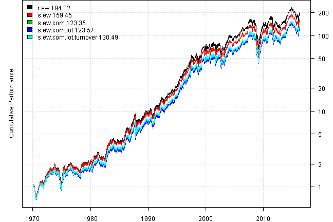

plot of chunk plot-6

print(plotbt.strategy.sidebyside(models, make.plot=F, return.table=T,perfromance.fn = engineering.returns.kpi))

	r.ew	s.ew	s.ew.com	s.ew.com.lot	s.ew.com.lot.turnover
Period	Jan1970 - May2016	Jan1970 - May2016	Jan1970 - May2016	Jan1970 - May2016	Jan1970 - May2016
Cagr	12.03	11.56	10.94	10.95	11.08
Sharpe	0.65	0.63	0.6	0.6	0.61
DVR	0.52	0.51	0.49	0.49	0.5
R2	0.8	0.81	0.81	0.81	0.82
Volatility	20.97	20.89	20.89	20.88	20.87
MaxDD	-60.67	-60.88	-60.9	-60.89	-60.84
Exposure	99.82	99.82	99.82	99.82	99.82
Win.Percent	100	55.62	55.62	55.25	56.73
Avg.Trade	1765.79	0.21	0.21	0.22	0.52
Profit.Factor	NaN	1.4	1.4	1.41	1.66
Num.Trades	5	2785	2785	2726	1167

Another erroneous feature of above approach is automatic reinvestment of dividends. The back-test so far was based on split and dividend adjusted prices. In reality, the dividends are deposited into account as cash and allocated during next re-balance. Let’s switch to raw, un-adjusted, prices and properly incorporate historical splits and dividends into back-test (s.ew.com.lot.turnover.unadjusted)

#*****************************************************************
# For each asset, append dividend and split columns
#****************************************************************** 	
data = env()
getSymbols.extra(tickers, src = 'yahoo', from = '1970-01-01', env = data, set.symbolnames = T, auto.assign = T)
	data.raw = data
#bt.unadjusted.add.div.split(data.raw)
bt.unadjusted.add.div.split(data.raw, infer.div.split.from.adjusted=T)
	
bt.prep(data.raw, align='remove.na', fill.gaps = T)

#*****************************************************************
# s.ew.com.lot.turnover.unadjusted
#******************************************************************
data.raw$weight[] = NA
	data.raw$weight[period.ends,] = weights
models$s.ew.com.lot.turnover.unadjusted = bt.run.share.ex(data.raw, clean.signal=F, silent=T, commission=commission, trade.summary=T,
	lot.size=100,
	control = list(round.lot = list(select = 'minimum.turnover', diff.target = 5/100)),
	adjusted = F
)

#*****************************************************************
# Create Report
#****************************************************************** 
plotbt(models, plotX = T, log = 'y', LeftMargin = 3, main = NULL)	    	
	mtext('Cumulative Performance', side = 2, line = 1)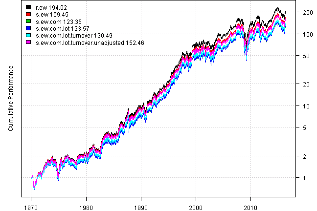

plot of chunk plot-7

print(plotbt.strategy.sidebyside(models, make.plot=F, return.table=T,perfromance.fn = engineering.returns.kpi))

	r.ew	s.ew	s.ew.com	s.ew.com.lot	s.ew.com.lot.turnover	s.ew.com.lot.turnover.unadjusted
Period	Jan1970 - May2016	Jan1970 - May2016	Jan1970 - May2016	Jan1970 - May2016	Jan1970 - May2016	Jan1970 - May2016
Cagr	12.03	11.56	10.94	10.95	11.08	11.45
Sharpe	0.65	0.63	0.6	0.6	0.61	0.63
DVR	0.52	0.51	0.49	0.49	0.5	0.51
R2	0.8	0.81	0.81	0.81	0.82	0.81
Volatility	20.97	20.89	20.89	20.88	20.87	20.74
MaxDD	-60.67	-60.88	-60.9	-60.89	-60.84	-60.68
Exposure	99.82	99.82	99.82	99.82	99.82	99.82
Win.Percent	100	55.62	55.62	55.25	56.73	54.34
Avg.Trade	1765.79	0.21	0.21	0.22	0.52	0.21
Profit.Factor	NaN	1.4	1.4	1.41	1.66	1.18
Num.Trades	5	2785	2785	2726	1167	1025

Another missing feature of above approach is taxes. In reality, unless you invest in tax sheltered account, the taxes are due at the end of the year. Let’s add tax event to the back-test on the last day in April each year (s.ew.com.lot.turnover.unadjusted.tax)

#*****************************************************************
# s.ew.com.lot.turnover.unadjusted.tax
#******************************************************************
data.raw$weight[] = NA
	data.raw$weight[period.ends,] = weights
models$s.ew.com.lot.turnover.unadjusted.tax = bt.run.share.ex(data.raw, clean.signal=F, silent=T, commission=commission, trade.summary=T,
	lot.size=100,
	control = list(round.lot = list(select = 'minimum.turnover', diff.target = 5/100)),
	adjusted = F,
	# enable taxes
	tax.control = default.tax.control(),
	cashflow.control = list(
		taxes = list(
			#cashflows = event.at(prices, 'year', offset=60),
			cashflows = event.at(prices, period.ends = custom.date.bus('last day in Apr', prices, 'UnitedStates/NYSE'), offset=0),
			cashflow.fn = tax.cashflows,
			invest = 'update',
			type = 'fee.rebate'
		)
	)
)



#*****************************************************************
# Create Report
#****************************************************************** 
plotbt(models, plotX = T, log = 'y', LeftMargin = 3, main = NULL)	    	
	mtext('Cumulative Performance', side = 2, line = 1)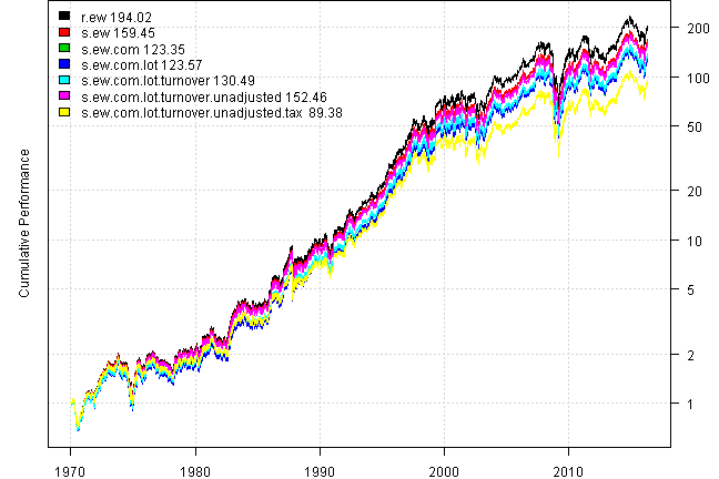

plot of chunk plot-8

print(plotbt.strategy.sidebyside(models, make.plot=F, return.table=T,perfromance.fn = engineering.returns.kpi))

	r.ew	s.ew	s.ew.com	s.ew.com.lot	s.ew.com.lot.turnover	s.ew.com.lot.turnover.unadjusted	s.ew.com.lot.turnover.unadjusted.tax
Period	Jan1970 - May2016	Jan1970 - May2016	Jan1970 - May2016	Jan1970 - May2016	Jan1970 - May2016	Jan1970 - May2016	Jan1970 - May2016
Cagr	12.03	11.56	10.94	10.95	11.08	11.45	10.17
Sharpe	0.65	0.63	0.6	0.6	0.61	0.63	0.57
DVR	0.52	0.51	0.49	0.49	0.5	0.51	0.48
R2	0.8	0.81	0.81	0.81	0.82	0.81	0.84
Volatility	20.97	20.89	20.89	20.88	20.87	20.74	20.78
MaxDD	-60.67	-60.88	-60.9	-60.89	-60.84	-60.68	-61.01
Exposure	99.82	99.82	99.82	99.82	99.82	99.82	99.82
Win.Percent	100	55.62	55.62	55.25	56.73	54.34	54.38
Avg.Trade	1765.79	0.21	0.21	0.22	0.52	0.21	0.21
Profit.Factor	NaN	1.4	1.4	1.41	1.66	1.18	1.19
Num.Trades	5	2785	2785	2726	1167	1025	1004

print('#Average Annual Portfolio Turnover')

#Average Annual Portfolio Turnover

layout(1)
barplot.with.labels(sapply(models, compute.turnover, data), 'Average Annual Portfolio Turnover')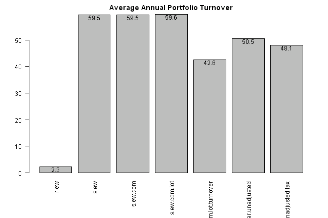

plot of chunk plot-8

m = models$s.ew.com.lot.turnover.unadjusted.tax

# aside plots
#plotbt.transition.map(m$weight, 'Tax')
#plota(make.xts(m$value,data$dates), type='l')
	

print('#Events for s.ew.com.lot.turnover.unadjusted.tax:')

#Events for s.ew.com.lot.turnover.unadjusted.tax:

print(to.nice(mlast(bt.make.trade.event.summary.table(m), 20),0))

	Type	MMM	AA	CAT	KO	HPQ	Cash	Com	Div	Value
2015-10-30	trade	11,300	165,400	24,400	39,800	62,300	19,598	0	0	8,419,187
2015-11-02	split	11,300	165,400	24,400	39,800	138,444	19,598	0	0	8,753,147
2015-11-04	dividend	11,300	165,400	24,400	39,800	138,444	24,560	0	4,962	8,818,726
2015-11-18	dividend	11,300	165,400	24,400	39,800	138,444	36,245	0	11,684	8,492,700
2015-11-27	dividend	11,300	165,400	24,400	39,800	138,444	49,418	0	13,174	8,577,156
2015-11-30	trade	11,300	165,400	24,400	39,800	138,444	49,418	0	0	8,571,946
2015-12-07	dividend	11,300	165,400	24,400	39,800	138,444	66,586	0	17,167	8,413,821
2015-12-31	trade	11,300	165,400	24,400	39,800	138,444	66,586	0	0	8,408,530
2016-01-15	dividend	11,300	165,400	24,400	39,800	138,444	84,886	0	18,300	7,305,544
2016-01-29	trade	10,000	207,500	24,300	35,200	155,800	8,706	705	0	7,567,415
2016-02-03	dividend	10,000	207,500	24,300	35,200	155,800	15,553	0	6,848	7,652,053
2016-02-10	dividend	10,000	207,500	24,300	35,200	155,800	26,563	0	11,010	7,569,199
2016-02-29	trade	10,500	185,300	24,400	38,300	154,800	16,272	319	0	8,276,707
2016-03-07	dividend	10,500	185,300	24,400	38,300	154,800	35,932	0	19,660	8,843,088
2016-03-11	dividend	10,500	185,300	24,400	38,300	154,800	49,413	0	13,482	8,831,849
2016-03-31	trade	10,500	185,300	24,400	38,300	154,800	49,413	0	0	9,125,651
2016-04-21	dividend	10,500	185,300	24,400	38,300	154,800	68,128	0	18,715	9,310,298
2016-04-29	trade	11,100	166,400	23,900	41,400	151,500	2,313	314	0	9,290,052
2016-05-04	dividend	11,100	166,400	23,900	41,400	151,500	7,305	0	4,992	8,959,110
2016-05-06	trade	11,100	166,400	23,900	41,400	151,500	7,305	0	0	8,938,077

# aside summaries 
#print(mlast(bt.make.cashflow.event.summary.table(m), 20))
#print(look.at.taxes(m)['2015'])
#print(tax.summary(m))

I feel a lot more comfortable with latest version of back-test result and corresponding statistics because it resembles reality.

There are still more issues that one might want to incorporate into their back-test settings. Here are few ideas:

if allocation is based on the signal, unlike the sample strategy above, you might want to add execution lag. i.e. signal is generated on the second to last day of the month and execution takes place on the last day of the month
consider various cash flows over the life of the back-test. for example,
- a young investor, in his 20’s, contributes 5% of initial capital each year for the first 10 years,
- next there are small withdrawals of 1% of initial capital each year for the next 30 years to cover family expenses,
- finally, in retirement stage the withdrawals raise to 5% of portfolio equity each year

In conclusion, do not blindly trust the back-test numbers and corresponding statistics, consider if back-test is actually a good simulation of real portfolio performance.

Please note that the supporting code for this post is still in development. If you want to experiment at your own risk, please sign up for a beta testing by filling up the contact form.

For your convenience, the 2015-10-19-Backtest-Reality-Check post source code.

Systematic Investor's Blog About Contact

Back-test Reality Check

Related Posts

RFinance 2016 15 May 2016

Benchmark Plus 14 Apr 2016

Exponentially Weighted Volatility using RCPP 10 Apr 2016