Adjusted Data
30 Mar 2015To install Systematic Investor Toolbox (SIT) please visit About page.
Date at DTR Trading wrote an excellent series on cons / pros of using Adjusted data for momentum strategies.
Below I will try to adapt a code from the posts:
#*****************************************************************
# Load historical end of day data
#*****************************************************************
library(SIT)
load.packages('quantmod')


tickers = '
AGG # iShares Barclays Aggregate Bond Fund
DBC # PowerShares DB Com Indx Trckng Fund
EEM # iShares MSCI Emerging Markets Indx
EFA # iShares MSCI EAFE Index Fund
GLD # SPDR Gold Trust
IYR # iShares Dow Jones US Real Estate
JNK # SPDR Barclays Capital High Yield Bond
PPH # Market Vectors Pharmaceutical
SPY # SPDR S&P 500 Trust
TIP # iShares Barclays TIPS Bond Fund
'

tickers = '
EEM # iShares MSCI Emerging Markets Index ETF
EFA # iShares MSCI EAFE Index ETF
FXI # iShares China Large#Cap ETF
IEF # iShares 7#10 Year Treasury Bond ETF
IYR # iShares Dow Jones US Real Estate ETF
SHY # iShares 1#3 Year Treasury Bond ETF
SPY # SPDR S&P 500 Trust ETF
TIP # iShares Barclays TIPS Bond ETF
XLV # Health Care Select Sector SPDR ETF
UUP # PowerShares DB US Dollar Bullish ETF
'

data = new.env()
getSymbols.extra(tickers, src = 'yahoo', from = '1970-01-01', env = data, set.symbolnames = T, auto.assign = T)
#print(bt.start.dates(data))
#*****************************************************************
# Contruct another back-test environment with split-adjusted prices, do not include dividends
# http://www.fintools.com/wp-content/uploads/2012/02/DividendAdjustedStockPrices.pdf
# http://www.pstat.ucsb.edu/research/papers/momentum.pdf
#
# For example of split and dividend schedule
# http://finance.yahoo.com/q/hp?s=EFA&g=v
#*****************************************************************
data.price = new.env()
data.price$symbolnames = data$symbolnames
  for(i in data$symbolnames) data.price[[i]] = adjustOHLC(data[[i]], symbol.name=i, adjust='split', use.Adjusted=F)
bt.prep(data.price, align='keep.all', dates='2002::', fill.gaps=T)

#*****************************************************************
# Adjust prices
#*****************************************************************
  for(i in data$symbolnames) data[[i]] = adjustOHLC(data[[i]], use.Adjusted=T)
bt.prep(data, align='keep.all', dates='2002::', fill.gaps=T)
We constructed two environments:
- data environment contains split and dividend adjusted prices
- data.price environment contains only split adjusted prices
#*****************************************************************
# Setup
#*****************************************************************
prices = data$prices
  n = ncol(prices)
  nperiods = nrow(prices)

frequency = 'months'
period.ends = endpoints(prices, frequency)
  period.ends1 = period.ends - 1 # lag by one day
  period.ends1 = period.ends1[period.ends1 > 0]
  period.ends0 = period.ends1 + 1

models = list()

commission = list(cps = 0.01, fixed = 10.0, percentage = 0.0)


#*****************************************************************
# 60 day rate of change for ranking
#******************************************************************
return = prices / mlag(prices,60) - 1
position.score = iif(return < 0, NA, return)

data$weight[] = NA
  data$weight[period.ends0,] = ntop(position.score[period.ends1,], 1)
models$mom60 = bt.run.share(data, clean.signal=F, commission = commission, trade.summary=T, silent=T)

# alternatively use do.lag
#data$weight[] = NA
#  data$weight[period.ends1,] = ntop(position.score[period.ends1,], 1)
#models$mom60A = bt.run.share(data, clean.signal=F, do.lag=2, commission = commission, trade.summary=T, silent=T)

#print(last.trades(models$mom60, make.plot=F, return.table=T))
#print(last.trades(models$mom60A, make.plot=F, return.table=T))

#*****************************************************************
# 60/120 day rate of change for ranking
#******************************************************************
return = prices / mlag(prices,60) - 1 + prices / mlag(prices,120) - 1
position.score = iif(return < 0, NA, return)

data$weight[] = NA
  data$weight[period.ends0,] = ntop(position.score[period.ends1,], 1)
models$mom120 = bt.run.share(data, clean.signal=F, commission = commission, trade.summary=T, silent=T)

#*****************************************************************
# Create Report
#*****************************************************************
#strategy.performance.snapshoot(models, T)
plotbt(models, plotX = T, log = 'y', LeftMargin = 3, main = NULL)
	mtext('Cumulative Performance', side = 2, line = 1)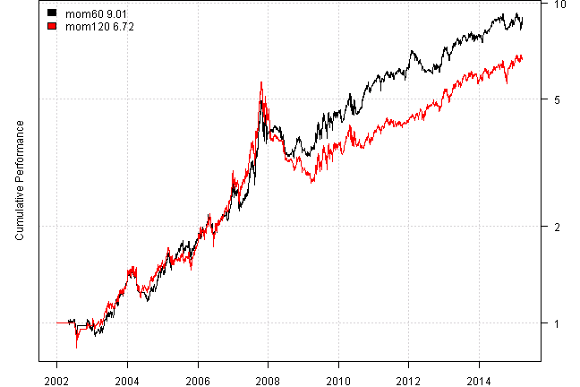
print(plotbt.strategy.sidebyside(models, make.plot=F, return.table=T, perfromance.fn=engineering.returns.kpi))| mom60 | mom120 | |
|---|---|---|
| Period | Jan2002 - Mar2015 | Jan2002 - Mar2015 |
| Cagr | 18.05 | 15.47 |
| Sharpe | 0.89 | 0.76 |
| DVR | 0.85 | 0.7 |
| R2 | 0.95 | 0.92 |
| Volatility | 21.26 | 22.21 |
| MaxDD | -33.49 | -51.75 |
| Exposure | 94.36 | 94.36 |
| Win.Percent | 63.76 | 62.42 |
| Avg.Trade | 1.69 | 1.49 |
| Profit.Factor | 2.24 | 2 |
| Num.Trades | 149 | 149 |
print(last.trades(models$mom60, make.plot=F, return.table=T))| models$mom60 | weight | entry.date | exit.date | nhold | entry.price | exit.price | return |
|---|---|---|---|---|---|---|---|
| SPY | 100 | 2013-06-28 | 2013-07-31 | 33 | 155.04 | 163.06 | 5.17 |
| XLV | 100 | 2013-07-31 | 2013-08-30 | 30 | 49.88 | 48.12 | -3.53 |
| XLV | 100 | 2013-08-30 | 2013-09-30 | 31 | 48.12 | 49.66 | 3.20 |
| FXI | 100 | 2013-09-30 | 2013-10-31 | 31 | 35.92 | 36.40 | 1.34 |
| EEM | 100 | 2013-10-31 | 2013-11-29 | 29 | 41.16 | 41.05 | -0.27 |
| XLV | 100 | 2013-11-29 | 2013-12-31 | 32 | 54.24 | 54.64 | 0.75 |
| SPY | 100 | 2013-12-31 | 2014-01-31 | 31 | 180.35 | 173.99 | -3.53 |
| XLV | 100 | 2014-01-31 | 2014-02-28 | 28 | 55.16 | 58.59 | 6.22 |
| IYR | 100 | 2014-02-28 | 2014-03-31 | 31 | 65.72 | 65.81 | 0.14 |
| IYR | 100 | 2014-03-31 | 2014-04-30 | 30 | 65.81 | 67.81 | 3.04 |
| EEM | 100 | 2014-04-30 | 2014-05-30 | 30 | 40.42 | 41.62 | 2.97 |
| EEM | 100 | 2014-05-30 | 2014-06-30 | 31 | 41.62 | 42.62 | 2.40 |
| IYR | 100 | 2014-06-30 | 2014-07-31 | 31 | 70.41 | 70.33 | -0.11 |
| FXI | 100 | 2014-07-31 | 2014-09-30 | 61 | 39.96 | 37.80 | -5.41 |
| UUP | 100 | 2014-09-30 | 2014-10-31 | 31 | 22.87 | 23.09 | 0.96 |
| XLV | 100 | 2014-10-31 | 2014-11-28 | 28 | 67.02 | 69.35 | 3.48 |
| XLV | 100 | 2014-11-28 | 2014-12-31 | 33 | 69.35 | 68.38 | -1.40 |
| IYR | 100 | 2014-12-31 | 2015-01-30 | 30 | 76.84 | 81.23 | 5.71 |
| IYR | 100 | 2015-01-30 | 2015-02-27 | 28 | 81.23 | 79.12 | -2.60 |
| FXI | 100 | 2015-02-27 | 2015-03-30 | 31 | 43.76 | 44.74 | 2.24 |
Next let’s consider following 3 setups:
- “Adjusted” - split and dividend adjusted price data. The signals and P&L are derived only from the adjusted data time series.
- “Actual” - using only split adjusted data, that has not been adjusted for dividends. The signals and P&L are derived only from the only split adjusted data time series.
- “Hybrid” - use “Actual” time series for signal generation and the “Adjusted” time series for the P&L calculation.
#*****************************************************************
# Helper function
#******************************************************************
run.strategy = function(prices , data, name) {
  models = list()

  return = prices / mlag(prices,60) - 1
  position.score = iif(return < 0, NA, return)

  data$weight[] = NA
    data$weight[period.ends0,] = ntop(position.score[period.ends1,], 1)
  models[[paste0('mom60',name)]] = bt.run.share(data, clean.signal=F, commission = commission, trade.summary=T, silent=T)


  return = prices / mlag(prices,60) - 1 + prices / mlag(prices,120) - 1
  position.score = iif(return < 0, NA, return)

  data$weight[] = NA
    data$weight[period.ends0,] = ntop(position.score[period.ends1,], 1)
  models[[paste0('mom120',name)]] = bt.run.share(data, clean.signal=F, commission = commission, trade.summary=T, silent=T)

  models
}

#*****************************************************************
# Setup
#******************************************************************
prices.adj = data$prices
prices.split = data.price$prices

all.models = list()
all.models = c(all.models, run.strategy(prices.adj, data, 'Adjusted'))
all.models = c(all.models, run.strategy(prices.split, data.price, 'Actual'))
all.models = c(all.models, run.strategy(prices.split, data, 'Hybrid'))

#*****************************************************************
# Create Report
#*****************************************************************
models = all.models[grep('mom60', names(all.models))]

plotbt(models, plotX = T, log = 'y', LeftMargin = 3, main = NULL)
	mtext('Cumulative Performance', side = 2, line = 1)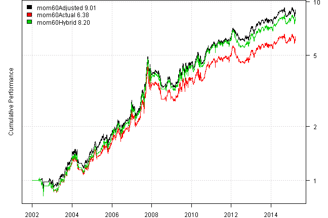
print(plotbt.strategy.sidebyside(models, make.plot=F, return.table=T, perfromance.fn=engineering.returns.kpi))| mom60Adjusted | mom60Actual | mom60Hybrid | |
|---|---|---|---|
| Period | Jan2002 - Mar2015 | Jan2002 - Mar2015 | Jan2002 - Mar2015 |
| Cagr | 18.05 | 15.02 | 17.22 |
| Sharpe | 0.89 | 0.76 | 0.85 |
| DVR | 0.85 | 0.73 | 0.82 |
| R2 | 0.95 | 0.96 | 0.96 |
| Volatility | 21.26 | 21.33 | 21.33 |
| MaxDD | -33.49 | -35.99 | -33.74 |
| Exposure | 94.36 | 92.44 | 92.44 |
| Win.Percent | 63.76 | 62.33 | 63.01 |
| Avg.Trade | 1.69 | 1.49 | 1.67 |
| Profit.Factor | 2.24 | 1.98 | 2.15 |
| Num.Trades | 149 | 146 | 146 |
models = all.models[grep('mom120', names(all.models))]

plotbt(models, plotX = T, log = 'y', LeftMargin = 3, main = NULL)
	mtext('Cumulative Performance', side = 2, line = 1)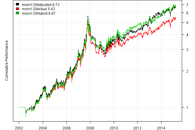
print(plotbt.strategy.sidebyside(models, make.plot=F, return.table=T, perfromance.fn=engineering.returns.kpi))| mom120Adjusted | mom120Actual | mom120Hybrid | |
|---|---|---|---|
| Period | Jan2002 - Mar2015 | Jan2002 - Mar2015 | Jan2002 - Mar2015 |
| Cagr | 15.47 | 13.61 | 15.66 |
| Sharpe | 0.76 | 0.69 | 0.77 |
| DVR | 0.7 | 0.64 | 0.73 |
| R2 | 0.92 | 0.92 | 0.94 |
| Volatility | 22.21 | 22.08 | 22.07 |
| MaxDD | -51.75 | -49.93 | -47.15 |
| Exposure | 94.36 | 92.47 | 92.47 |
| Win.Percent | 62.42 | 60.96 | 61.64 |
| Avg.Trade | 1.49 | 1.37 | 1.54 |
| Profit.Factor | 2 | 1.9 | 2.02 |
| Num.Trades | 149 | 146 | 146 |
In agreement with source Adjusted and Hybrid outperform Actual.
(this report was produced on: 2015-03-31)