XIV Seasonality
02 Dec 2014To install Systematic Investor Toolbox (SIT) please visit About page.
A New (Better?) Measure of Risk and Uncertainty: The Volatility of Acceleration Volatility of Acceleration Part Two
Load historical data for SPY.
	#*****************************************************************
	# Load historical data
	#*****************************************************************
	library(SIT)
	load.packages('quantmod')

	tickers = spl('SPY')

	data <- new.env()
	getSymbols(tickers, src = 'yahoo', from = '1970-01-01', env = data, auto.assign = T)
		for(i in ls(data)) data[[i]] = adjustOHLC(data[[i]], use.Adjusted=T)
	bt.prep(data, align='remove.na')
Next let’s compute statistics and trading signal.
	price = data$prices$SPY
	ret = price / mlag(price) - 1
	ret = diff(log(price))

	vol = runSD(ret, 10)
	vol1 = SMA(abs(ret), 20)

	# VOA = volatility of acceleration
	# VOA= average of: | ln(pt/pt-1)- ln(pt-1/pt-2) |... | ln(pt-n/pt-n-1)|
	# VOA is the average of the absolute value of the first difference of daily log returns
	voa = SMA(abs(diff(ret)), 10)
	voa1 = runSD(diff(ret), 10)

# this look like MAD

	# Forecast VOA (F-VOA)= VOA(t)+ k*(VOA(t)- VOA(t-1))
	fvoa = voa + (voa - mlag(voa))


	plota(voa['2008:01::2008:10'], type='l', col='orange', lwd=2)
	plota.lines(vol['2008:01::2008:10'], col='blue', lwd=2)
	plota.lines(fvoa['2008:01::2008:10'], col='green', lwd=2)
	plota.legend(spl('Volatlity,Volatlity of Acceleration'), spl('orange,blue'))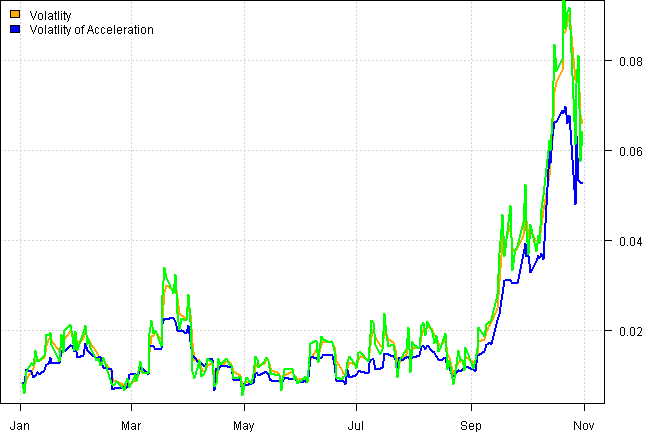
Note, check ?filter
Now we ready to back-test our strategy:
	#*****************************************************************
	# Code Strategies
	#*****************************************************************
	models = list()

	data$weight[] = NA
		data$weight[] = 1
	models$strategy = bt.run.share(data, clean.signal=F, silent=T)

	#*****************************************************************
	# standard volatility position sizing.
	# In this case we use the same 10-day measure for both and a 1% daily target risk
	#(1.5% for volatility of acceleration to reflect difference in scale)
	#*****************************************************************
	weight = 0.01/(vol *sqrt(1) )

	data$weight[] = NA
		data$weight[] = weight
	models$VOL = bt.run.share(data, clean.signal=F, silent=T)

	weight = 0.015/(voa *sqrt(1) )

	data$weight[] = NA
		data$weight[] = weight
	models$VOA = bt.run.share(data, clean.signal=F, silent=T)

	weight = 0.015/(fvoa *sqrt(1) )

	data$weight[] = NA
		data$weight[] = weight
	models$FVOA = bt.run.share(data, clean.signal=F, silent=T)
and create reports
Create Report:
	#*****************************************************************
	# Create Report
	#*****************************************************************
	plotbt(models, plotX = T, log = 'y', LeftMargin = 3, main = NULL)
		mtext('Cumulative Performance', side = 2, line = 1)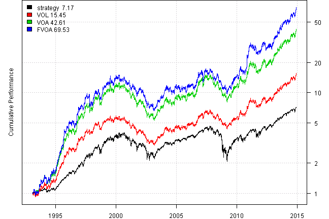
print(plotbt.strategy.sidebyside(models, make.plot=F, return.table=T))| strategy | VOL | VOA | FVOA | |
|---|---|---|---|---|
| Period | Jan1993 - Dec2014 | Jan1993 - Dec2014 | Jan1993 - Dec2014 | Jan1993 - Dec2014 |
| Cagr | 9.43 | 13.34 | 18.72 | 21.41 |
| Sharpe | 0.57 | 0.78 | 0.83 | 0.87 |
| DVR | 0.42 | 0.56 | 0.56 | 0.55 |
| Volatility | 19.05 | 18.33 | 24.32 | 26.45 |
| MaxDD | -55.19 | -49.21 | -57.73 | -56.34 |
| AvgDD | -2.06 | -3.2 | -4.15 | -4.6 |
| VaR | -1.89 | -1.84 | -2.42 | -2.46 |
| CVaR | -2.83 | -2.69 | -3.54 | -3.76 |
| Exposure | 99.98 | 99.8 | 99.78 | 99.76 |
(this report was produced on: 2014-12-07)