Quantitative Approach To Tactical Asset Allocation Strategy + Bands
To install Systematic Investor Toolbox (SIT) please visit About page.
Following is the modified version of the Quantitative Approach To Tactical Asset Allocation Strategy(QATAA) by Mebane T. Faber backtest. For more details please see SSRN paper
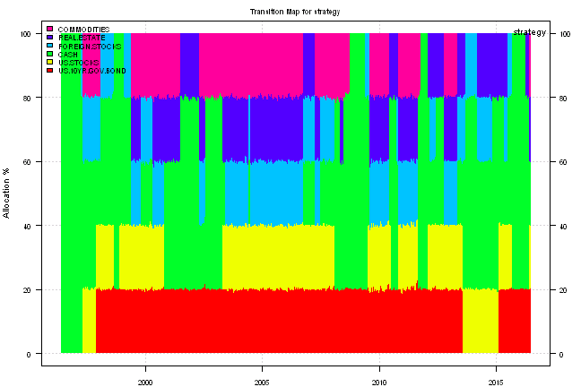
The QATAA Strategy allocates 20% across 5 asset classes:
- US Stocks
- Foreign Stocks
- US 10YR Government Bonds
- Real Estate
- Commodities
In the original strategy, if asset is above it’s 10 month moving average it gets 20% allocation; otherwise, it’s weight is allocated to cash. The re-balancing process is done Monthly.
We introduce +5%/-5% bands around the 10 month moving average to avoid whipsaws. The strategy is invested if asset crosses upper band and goes to cash if asset drops below the lower band.
Following report is based on Monthly re-balancing, signal is generated one day before the month end, and execution is done at close at the month end.
The transaction cost is assumed 1cps + $10 per transaction
Load historical data from Yahoo Finance:
#*****************************************************************
# Load historical data
#*****************************************************************
library(SIT)
load.packages('quantmod')

tickers = '
US.STOCKS = VTI + VTSMX
FOREIGN.STOCKS = VEU + FDIVX
US.10YR.GOV.BOND = IEF + VFITX
REAL.ESTATE = VNQ + VGSIX
COMMODITIES = DBC + CRB
CASH = BND + VBMFX
'

# load saved Proxies Raw Data, data.proxy.raw
load('data.proxy.raw.Rdata')

data <- new.env()

getSymbols.extra(tickers, src = 'yahoo', from = '1970-01-01', env = data, raw.data = data.proxy.raw, auto.assign = T, set.symbolnames = T, getSymbols.fn = getSymbols.fn, calendar=calendar)
  for(i in data$symbolnames) data[[i]] = adjustOHLC(data[[i]], use.Adjusted=T)
bt.prep(data, align='remove.na', dates='::')

print(last(data$prices))| US.STOCKS | FOREIGN.STOCKS | US.10YR.GOV.BOND | REAL.ESTATE | COMMODITIES | CASH | |
|---|---|---|---|---|---|---|
| 2016-06-24 | 104.05 | 41.22 | 112.21 | 84.86 | 15.01 | 83.7 |
#*****************************************************************
# Setup
#*****************************************************************
data$universe = data$prices > 0
	# do not allocate to CASH
	data$universe$CASH = NA

prices = data$prices * data$universe
	n = ncol(prices)
Code Strategy Rules:
#*****************************************************************
# Code Strategy
#******************************************************************
sma = bt.apply.matrix(prices, SMA, 200)

# check price cross over with +5%/-5% bands
signal = iif(cross.up(prices, sma * 1.05), 1, iif(cross.dn(prices, sma * 0.95), 0, NA))
signal = ifna(bt.apply.matrix(signal, ifna.prev),0)

# If asset is above it's 10 month moving average it gets 20% allocation
#weight = iif(prices > sma, 20/100, 0)
weight = iif(signal == 1, 20/100, 0)

# otherwise, it's weight is allocated to cash
weight$CASH = 1 - rowSums(weight)


obj$weights$strategy = weight[period.ends,]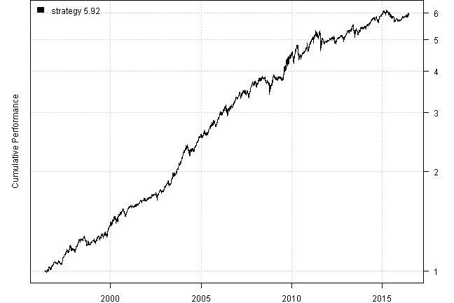
#Strategy Performance:
| strategy | |
|---|---|
| Period | May1996 - Jun2016 |
| Cagr | 9.24 |
| Sharpe | 1.18 |
| DVR | 1.15 |
| R2 | 0.97 |
| Volatility | 7.78 |
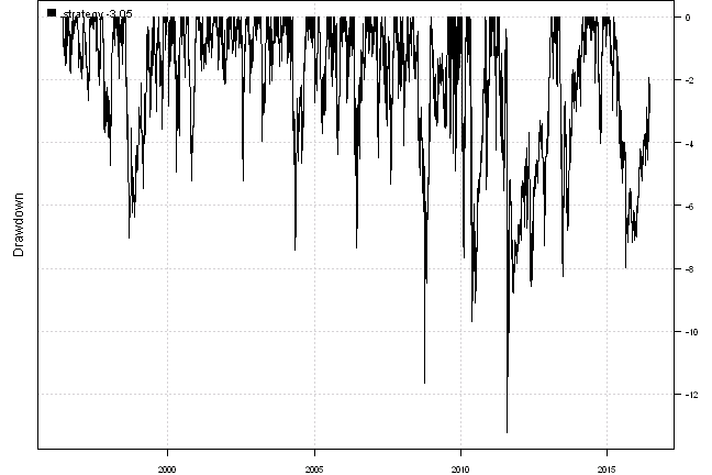
| MaxDD | -13.24 |
| Exposure | 99.72 |
| Win.Percent | 63.85 |
| Avg.Trade | 0.2 |
| Profit.Factor | 2.07 |
| Num.Trades | 960 |
#Monthly Results for strategy :
| Jan | Feb | Mar | Apr | May | Jun | Jul | Aug | Sep | Oct | Nov | Dec | Year | MaxDD | |
|---|---|---|---|---|---|---|---|---|---|---|---|---|---|---|
| 1996 | 1.3 | 0.2 | -0.2 | 1.7 | 2.2 | 1.7 | -0.9 | 6.2 | -1.8 | |||||
| 1997 | 0.2 | 0.1 | -1.0 | 1.2 | 3.6 | 1.4 | 3.8 | -2.2 | 3.5 | -1.0 | -0.4 | 0.2 | 9.5 | -3.8 |
| 1998 | 1.1 | 2.4 | 2.1 | 1.1 | 0.0 | 1.1 | -0.1 | -4.7 | 2.3 | -0.6 | 0.3 | 1.6 | 6.3 | -7.0 |
| 1999 | 1.3 | -2.7 | 2.0 | 2.1 | -1.8 | 3.1 | -0.6 | 1.0 | 0.1 | 0.9 | 3.2 | 4.6 | 13.6 | -3.6 |
| 2000 | -1.3 | 3.1 | 1.9 | -2.7 | 0.9 | 3.4 | 0.3 | 3.3 | -1.2 | -2.1 | 2.4 | 2.2 | 10.5 | -5.2 |
| 2001 | 1.1 | 0.1 | -0.5 | 0.8 | 0.2 | 0.5 | 1.4 | 1.6 | 0.2 | 0.9 | -0.1 | -0.2 | 5.9 | -2.2 |
| 2002 | 0.5 | 1.1 | -0.1 | 1.6 | 0.8 | 0.8 | -2.5 | 2.4 | 2.3 | -0.8 | -0.4 | 3.3 | 9.3 | -5.2 |
| 2003 | 1.5 | 2.3 | -1.8 | 0.1 | 4.2 | 1.2 | 1.2 | 2.4 | 1.8 | 2.9 | 1.7 | 4.4 | 24.0 | -4.0 |
| 2004 | 2.4 | 3.1 | 1.7 | -5.1 | 2.5 | -0.2 | -0.4 | 2.2 | 2.3 | 2.5 | 2.6 | 1.8 | 16.2 | -7.4 |
| 2005 | -2.0 | 3.0 | -0.5 | -0.4 | 1.7 | 2.1 | 3.4 | 1.2 | 1.0 | -3.0 | 2.5 | 2.5 | 11.7 | -4.4 |
| 2006 | 4.5 | -1.0 | 2.4 | 1.6 | -2.3 | 0.7 | 1.6 | 1.3 | 0.2 | 2.8 | 2.5 | 0.0 | 15.1 | -7.3 |
| 2007 | 2.2 | -0.3 | 0.3 | 1.8 | 1.0 | -2.0 | 0.0 | 0.6 | 4.0 | 3.7 | -0.9 | 0.9 | 11.6 | -5.3 |
| 2008 | -1.3 | 2.5 | 0.3 | 0.5 | 0.5 | 0.2 | -1.8 | -0.5 | -2.4 | -2.6 | 4.7 | 5.1 | 4.8 | -11.6 |
| 2009 | -2.5 | -0.6 | 1.5 | -0.2 | 0.1 | -0.2 | 4.3 | 3.5 | 3.4 | -0.7 | 4.7 | 1.4 | 15.3 | -4.9 |
| 2010 | -4.1 | 2.9 | 4.3 | 2.6 | -6.3 | -1.1 | 2.6 | 1.3 | 0.8 | 1.7 | -1.4 | 5.2 | 8.1 | -9.7 |
| 2011 | 1.9 | 3.0 | 0.2 | 4.0 | -1.2 | -2.2 | 0.9 | -3.3 | -2.1 | -0.2 | 0.0 | 1.3 | 2.1 | -13.2 |
| 2012 | 0.6 | 0.4 | 1.0 | 0.8 | -3.7 | 1.8 | 1.3 | 0.5 | 0.1 | -1.3 | 1.0 | 1.5 | 3.9 | -5.1 |
| 2013 | 2.5 | -0.5 | 1.6 | 1.9 | -2.4 | -2.3 | 2.2 | -2.8 | 2.9 | 2.0 | 0.4 | 0.4 | 5.9 | -8.3 |
| 2014 | -0.9 | 2.3 | 0.2 | 1.2 | 1.7 | 1.1 | -0.8 | 2.1 | -2.9 | 2.8 | 1.4 | 0.4 | 8.7 | -4.0 |
| 2015 | 2.2 | -0.6 | 0.5 | -1.4 | -0.2 | -2.4 | 0.9 | -2.9 | 0.8 | -0.1 | -0.4 | -0.3 | -4.1 | -8.0 |
| 2016 | 1.6 | 1.0 | 0.5 | -0.4 | 0.4 | 1.0 | 4.0 | -1.7 | ||||||
| Avg | 0.6 | 1.1 | 0.8 | 0.5 | 0.0 | 0.4 | 0.9 | 0.3 | 0.9 | 0.5 | 1.3 | 1.8 | 9.0 | -5.9 |
#Trades for strategy :
| strategy | weight | entry.date | exit.date | nhold | entry.price | exit.price | return |
|---|---|---|---|---|---|---|---|
| CASH | 80 | 2015-10-30 | 2015-11-30 | 31 | 80.89 | 80.57 | -0.31 |
| US.10YR.GOV.BOND | 20 | 2015-11-30 | 2015-12-31 | 31 | 105.29 | 104.82 | -0.09 |
| CASH | 80 | 2015-11-30 | 2015-12-31 | 31 | 80.57 | 80.43 | -0.14 |
| US.10YR.GOV.BOND | 20 | 2015-12-31 | 2016-01-29 | 29 | 104.82 | 108.31 | 0.67 |
| CASH | 80 | 2015-12-31 | 2016-01-29 | 29 | 80.43 | 81.39 | 0.96 |
| US.10YR.GOV.BOND | 20 | 2016-01-29 | 2016-02-29 | 31 | 108.31 | 109.92 | 0.3 |
| CASH | 80 | 2016-01-29 | 2016-02-29 | 31 | 81.39 | 82.09 | 0.68 |
| US.10YR.GOV.BOND | 20 | 2016-02-29 | 2016-03-31 | 31 | 109.92 | 109.85 | -0.01 |
| CASH | 80 | 2016-02-29 | 2016-03-31 | 31 | 82.09 | 82.65 | 0.54 |
| US.10YR.GOV.BOND | 20 | 2016-03-31 | 2016-04-29 | 29 | 109.85 | 109.68 | -0.03 |
| REAL.ESTATE | 20 | 2016-03-31 | 2016-04-29 | 29 | 83.05 | 81.1 | -0.47 |
| CASH | 60 | 2016-03-31 | 2016-04-29 | 29 | 82.65 | 82.81 | 0.12 |
| US.10YR.GOV.BOND | 20 | 2016-04-29 | 2016-05-31 | 32 | 109.68 | 109.57 | -0.02 |
| REAL.ESTATE | 20 | 2016-04-29 | 2016-05-31 | 32 | 81.1 | 82.92 | 0.45 |
| CASH | 60 | 2016-04-29 | 2016-05-31 | 32 | 82.81 | 82.8 | 0 |
| US.STOCKS | 20 | 2016-05-31 | 2016-06-24 | 24 | 107.34 | 104.05 | -0.61 |
| US.10YR.GOV.BOND | 20 | 2016-05-31 | 2016-06-24 | 24 | 109.57 | 112.21 | 0.48 |
| REAL.ESTATE | 20 | 2016-05-31 | 2016-06-24 | 24 | 82.92 | 84.86 | 0.47 |
| COMMODITIES | 20 | 2016-05-31 | 2016-06-24 | 24 | 14.71 | 15.01 | 0.41 |
| CASH | 20 | 2016-05-31 | 2016-06-24 | 24 | 82.8 | 83.7 | 0.22 |
#Signals for strategy :
| US.STOCKS | FOREIGN.STOCKS | US.10YR.GOV.BOND | REAL.ESTATE | COMMODITIES | CASH | |
|---|---|---|---|---|---|---|
| 2014-10-30 | 20 | 0 | 0 | 20 | 0 | 60 |
| 2014-11-26 | 20 | 0 | 0 | 20 | 0 | 60 |
| 2014-12-30 | 20 | 0 | 0 | 20 | 0 | 60 |
| 2015-01-29 | 20 | 0 | 20 | 20 | 0 | 40 |
| 2015-02-26 | 20 | 0 | 20 | 20 | 0 | 40 |
| 2015-03-30 | 20 | 0 | 20 | 20 | 0 | 40 |
| 2015-04-29 | 20 | 20 | 20 | 20 | 0 | 20 |
| 2015-05-28 | 20 | 20 | 20 | 20 | 0 | 20 |
| 2015-06-29 | 20 | 20 | 20 | 0 | 0 | 40 |
| 2015-07-30 | 20 | 20 | 20 | 0 | 0 | 40 |
| 2015-08-28 | 0 | 0 | 20 | 0 | 0 | 80 |
| 2015-09-29 | 0 | 0 | 20 | 0 | 0 | 80 |
| 2015-10-29 | 0 | 0 | 20 | 0 | 0 | 80 |
| 2015-11-27 | 0 | 0 | 20 | 0 | 0 | 80 |
| 2015-12-30 | 0 | 0 | 20 | 0 | 0 | 80 |
| 2016-01-28 | 0 | 0 | 20 | 0 | 0 | 80 |
| 2016-02-26 | 0 | 0 | 20 | 0 | 0 | 80 |
| 2016-03-30 | 0 | 0 | 20 | 20 | 0 | 60 |
| 2016-04-28 | 0 | 0 | 20 | 20 | 0 | 60 |
| 2016-05-27 | 20 | 0 | 20 | 20 | 20 | 20 |
For your convenience, the Strategy-TAA-BANDS report can also be downloaded and viewed the pdf format.
(this report was produced on: 2016-06-25)