Elastic Asset Allocation Strategy
To install Systematic Investor Toolbox (SIT) please visit About page.
The Elastic Asset Allocation Strategy(EAA) backtest and live signal. For more details please see SSRN paper
The EAA Strategy uses a geometrical weighted average of the historical returns, volatilities and correlations, using elasticities as weights:
asset’s attractivness = [return ^ wR] * [(1-correlation) ^ wC] / [volatility ^ wV]
where:
- return is average asset’s return over last year using different timeframes
- correlation is asset’s correlation with equal weight, market, index
- volatility is asset’s historical volatility
- wR, wC, wV are user elasticities
Load historical data from Yahoo Finance:
#*****************************************************************
# Load historical data
#*****************************************************************
library(SIT)
load.packages('quantmod')

tickers = '
US.STOCKS = VTI + VTSMX
FOREIGN.STOCKS = VEU + FDIVX
EMERGING.MARKETS=EEM + VEIEX
US.10YR.GOV.BOND = IEF + VFITX
REAL.ESTATE = VNQ + VGSIX
COMMODITIES = DBC + CRB
CASH = BND + VBMFX
'

# load saved Proxies Raw Data, data.proxy.raw
load('data.proxy.raw.Rdata')

data <- new.env()

getSymbols.extra(tickers, src = 'yahoo', from = '1970-01-01', env = data, raw.data = data.proxy.raw, auto.assign = T, set.symbolnames = T, getSymbols.fn = getSymbols.fn, calendar=calendar)
  for(i in data$symbolnames) data[[i]] = adjustOHLC(data[[i]], use.Adjusted=T)
bt.prep(data, align='remove.na', dates='::')

print(last(data$prices))| US.STOCKS | FOREIGN.STOCKS | EMERGING.MARKETS | US.10YR.GOV.BOND | REAL.ESTATE | COMMODITIES | CASH | |
|---|---|---|---|---|---|---|---|
| 2016-06-24 | 104.05 | 41.22 | 32.65 | 112.21 | 84.86 | 15.01 | 83.7 |
#*****************************************************************
# Setup
#*****************************************************************
data$universe = data$prices > 0
	# do not allocate to CASH
	data$universe$CASH = NA

prices = data$prices * data$universe
	n = ncol(prices)
Code Strategy Rules:
#*****************************************************************
# Code Strategy
#******************************************************************
ret = diff(log(prices))

n.top = 3

mom.lookback = 80
vol.lookback = 12*22
cor.lookback = 12*22

weight=list(r=1, v=0, c=0.5, s=2)

hist.vol = sqrt(252) * bt.apply.matrix(ret, runSD, n = vol.lookback)

#mean of cumulative returns of 1, 3, 6, and 12 month periods
mom = (prices / mlag(prices, 22)-1 + prices / mlag(prices, 3*22)-1
+ prices / mlag(prices, 6*22)-1 + prices / mlag(prices, 12 * 22)-1)/22

mkt.ret = rowMeans(ret, na.rm=T)

#*****************************************************************
# Compute Correlation to Market
#******************************************************************
mkt.cor = data$weight * NA
for(i in period.ends[period.ends > cor.lookback]){
  index = (i - cor.lookback):i
  hist = ret[index,]
    include.index = !is.na(colSums(hist))

  if(any(include.index))
  	mkt.cor[i,include.index] = cor(hist[,include.index], mkt.ret[index], use='complete.obs',method='pearson')
}

avg.rank = (mom^weight$r * (1 - mkt.cor)^weight$c / hist.vol^weight$v) ^ weight$s
meta.rank = br.rank(avg.rank[period.ends,])

#absolute momentum filter
weight = (meta.rank <= n.top)/rowSums(meta.rank <= n.top, na.rm=T) * (mom[period.ends,] > 0)

# otherwise, it's weight is allocated to cash
weight$CASH = 1 - rowSums(weight,na.rm=T)

obj$weights$strategy = weight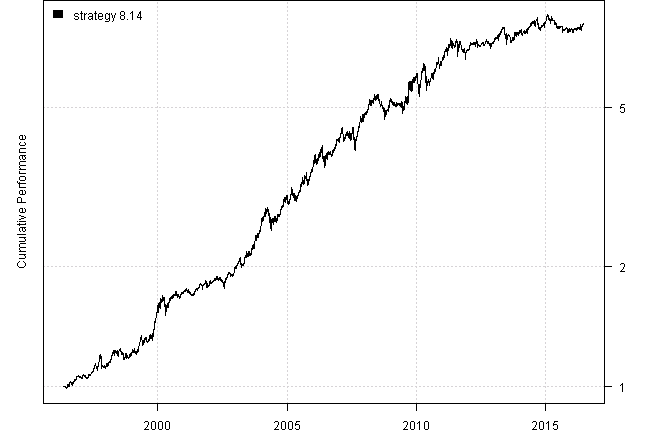
#Strategy Performance:
| strategy | |
|---|---|
| Period | May1996 - Jun2016 |
| Cagr | 10.98 |
| Sharpe | 1.03 |
| DVR | 0.99 |
| R2 | 0.96 |
| Volatility | 10.66 |
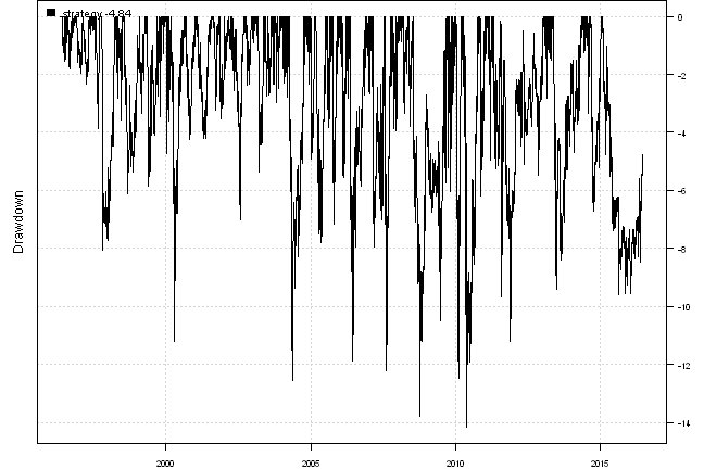
| MaxDD | -14.18 |
| Exposure | 99.72 |
| Win.Percent | 62.77 |
| Avg.Trade | 0.35 |
| Profit.Factor | 2.03 |
| Num.Trades | 658 |
#Monthly Results for strategy :
| Jan | Feb | Mar | Apr | May | Jun | Jul | Aug | Sep | Oct | Nov | Dec | Year | MaxDD | |
|---|---|---|---|---|---|---|---|---|---|---|---|---|---|---|
| 1996 | 1.3 | 0.2 | -0.2 | 1.7 | 2.2 | 1.7 | -0.9 | 6.2 | -1.8 | |||||
| 1997 | 0.2 | 0.1 | -1.0 | 1.5 | 0.9 | 1.0 | 4.5 | -3.5 | 7.3 | -3.9 | -1.0 | 1.6 | 7.4 | -8.1 |
| 1998 | 0.1 | 2.2 | 3.3 | 1.5 | -0.6 | 1.2 | -0.6 | -4.0 | 2.5 | -0.6 | 0.2 | 2.4 | 7.6 | -6.1 |
| 1999 | 1.7 | -2.9 | 1.6 | 6.7 | -3.3 | 3.6 | -1.8 | 1.4 | 1.9 | 1.5 | 7.0 | 10.5 | 30.6 | -5.8 |
| 2000 | -2.1 | 4.8 | -0.2 | -5.0 | 2.6 | 3.5 | 1.0 | 2.4 | -0.9 | -1.5 | 3.0 | 0.9 | 8.3 | -11.2 |
| 2001 | 0.7 | -0.4 | -1.4 | -0.8 | 1.0 | 2.2 | 0.9 | 1.9 | -0.3 | 1.8 | -1.7 | 0.1 | 4.1 | -4.2 |
| 2002 | 1.1 | 1.3 | 0.7 | 0.2 | 0.1 | -1.3 | -0.9 | 2.9 | 2.8 | -0.9 | -0.5 | 4.1 | 10.0 | -7.0 |
| 2003 | 2.5 | 3.0 | -2.8 | -0.4 | 4.6 | 0.5 | 0.6 | 4.3 | 0.4 | 5.3 | 1.1 | 6.8 | 28.7 | -5.4 |
| 2004 | 3.1 | 4.3 | 2.5 | -8.4 | 1.9 | -0.4 | 0.2 | 2.7 | 2.0 | 3.2 | 4.7 | 1.4 | 18.0 | -12.6 |
| 2005 | -3.5 | 6.6 | -2.0 | -3.1 | 1.7 | 3.0 | 6.3 | 1.0 | 3.8 | -4.7 | 3.1 | 3.7 | 16.3 | -7.8 |
| 2006 | 8.9 | -3.6 | 3.6 | 2.4 | -4.8 | 1.1 | 2.8 | 0.5 | -0.8 | 3.3 | 3.4 | 2.0 | 19.7 | -11.9 |
| 2007 | 3.2 | -2.3 | -0.6 | 1.4 | 0.8 | -1.6 | -1.4 | 0.7 | 4.0 | 8.9 | -1.4 | 1.7 | 13.8 | -12.2 |
| 2008 | 2.5 | 4.1 | 0.2 | 1.0 | 2.7 | 0.7 | -3.0 | -1.4 | -3.7 | -2.3 | 3.9 | 5.1 | 9.9 | -13.8 |
| 2009 | -2.7 | -0.7 | 1.1 | -0.6 | -0.3 | -1.3 | 4.5 | 0.8 | 7.4 | -2.6 | 5.7 | 2.0 | 13.5 | -7.7 |
| 2010 | -7.1 | 2.8 | 8.2 | 1.7 | -7.6 | -0.3 | 3.7 | -0.4 | 5.3 | 3.0 | -1.1 | 3.6 | 11.3 | -14.2 |
| 2011 | 2.9 | 4.2 | 0.5 | 4.4 | -1.7 | -2.7 | 3.1 | -0.5 | -4.0 | -0.4 | -1.3 | 1.4 | 5.6 | -11.2 |
| 2012 | 2.6 | 0.6 | 0.6 | 1.5 | -2.7 | -0.1 | 1.5 | 0.0 | 0.1 | -1.1 | 0.5 | 1.3 | 4.7 | -5.0 |
| 2013 | 1.9 | 0.3 | 2.4 | 3.2 | -3.7 | -2.4 | 2.1 | -3.7 | 2.0 | 2.8 | 0.9 | 1.2 | 6.9 | -9.4 |
| 2014 | -2.5 | 1.9 | 0.5 | 1.5 | 1.0 | 1.8 | -1.2 | 3.3 | -5.4 | 1.6 | 1.3 | 0.6 | 4.2 | -6.7 |
| 2015 | 4.5 | -2.5 | 0.3 | -2.3 | -1.2 | -1.5 | 1.1 | -2.2 | 0.6 | 0.0 | -0.5 | 0.5 | -3.4 | -9.6 |
| 2016 | -0.4 | 0.8 | 0.4 | -0.8 | 1.2 | 1.9 | 3.2 | -3.0 | ||||||
| Avg | 0.9 | 1.2 | 0.9 | 0.3 | -0.4 | 0.5 | 1.2 | 0.3 | 1.3 | 0.8 | 1.4 | 2.5 | 10.8 | -8.3 |
#Trades for strategy :
| strategy | weight | entry.date | exit.date | nhold | entry.price | exit.price | return |
|---|---|---|---|---|---|---|---|
| CASH | 100 | 2015-08-31 | 2015-09-30 | 30 | 80.38 | 80.87 | 0.6 |
| CASH | 100 | 2015-09-30 | 2015-10-30 | 30 | 80.87 | 80.89 | 0.03 |
| REAL.ESTATE | 33.3 | 2015-10-30 | 2015-11-30 | 31 | 77.22 | 76.74 | -0.21 |
| CASH | 66.7 | 2015-10-30 | 2015-11-30 | 31 | 80.89 | 80.57 | -0.26 |
| REAL.ESTATE | 33.3 | 2015-11-30 | 2015-12-31 | 31 | 76.74 | 78.14 | 0.61 |
| CASH | 66.7 | 2015-11-30 | 2015-12-31 | 31 | 80.57 | 80.43 | -0.12 |
| REAL.ESTATE | 33.3 | 2015-12-31 | 2016-01-29 | 29 | 78.14 | 75.46 | -1.15 |
| CASH | 66.7 | 2015-12-31 | 2016-01-29 | 29 | 80.43 | 81.39 | 0.8 |
| CASH | 100 | 2016-01-29 | 2016-02-29 | 31 | 81.39 | 82.09 | 0.85 |
| US.10YR.GOV.BOND | 33.3 | 2016-02-29 | 2016-03-31 | 31 | 109.92 | 109.85 | -0.02 |
| CASH | 66.7 | 2016-02-29 | 2016-03-31 | 31 | 82.09 | 82.65 | 0.45 |
| US.10YR.GOV.BOND | 33.3 | 2016-03-31 | 2016-04-29 | 29 | 109.85 | 109.68 | -0.05 |
| REAL.ESTATE | 33.3 | 2016-03-31 | 2016-04-29 | 29 | 83.05 | 81.1 | -0.78 |
| CASH | 33.3 | 2016-03-31 | 2016-04-29 | 29 | 82.65 | 82.81 | 0.06 |
| US.STOCKS | 33.3 | 2016-04-29 | 2016-05-31 | 32 | 105.51 | 107.34 | 0.58 |
| US.10YR.GOV.BOND | 33.3 | 2016-04-29 | 2016-05-31 | 32 | 109.68 | 109.57 | -0.03 |
| REAL.ESTATE | 33.3 | 2016-04-29 | 2016-05-31 | 32 | 81.1 | 82.92 | 0.75 |
| US.10YR.GOV.BOND | 33.3 | 2016-05-31 | 2016-06-24 | 24 | 109.57 | 112.21 | 0.8 |
| REAL.ESTATE | 33.3 | 2016-05-31 | 2016-06-24 | 24 | 82.92 | 84.86 | 0.78 |
| CASH | 33.3 | 2016-05-31 | 2016-06-24 | 24 | 82.8 | 83.7 | 0.36 |
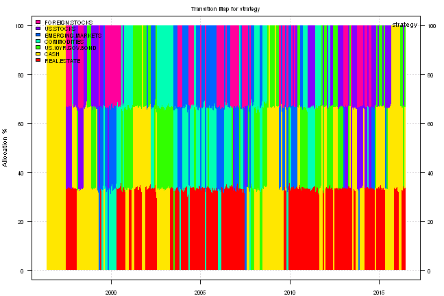
#Signals for strategy :
| US.STOCKS | FOREIGN.STOCKS | EMERGING.MARKETS | US.10YR.GOV.BOND | REAL.ESTATE | COMMODITIES | CASH | |
|---|---|---|---|---|---|---|---|
| 2014-10-30 | 0 | 0 | 0 | 33 | 33 | 0 | 33 |
| 2014-11-26 | 33 | 0 | 0 | 0 | 33 | 0 | 33 |
| 2014-12-30 | 0 | 0 | 0 | 33 | 33 | 0 | 33 |
| 2015-01-29 | 0 | 0 | 0 | 33 | 33 | 0 | 33 |
| 2015-02-26 | 33 | 0 | 0 | 0 | 33 | 0 | 33 |
| 2015-03-30 | 0 | 0 | 0 | 33 | 33 | 0 | 33 |
| 2015-04-29 | 33 | 0 | 33 | 0 | 0 | 0 | 33 |
| 2015-05-28 | 33 | 0 | 0 | 33 | 0 | 0 | 33 |
| 2015-06-29 | 33 | 0 | 0 | 0 | 0 | 0 | 67 |
| 2015-07-30 | 33 | 0 | 0 | 0 | 0 | 0 | 67 |
| 2015-08-28 | 0 | 0 | 0 | 0 | 0 | 0 | 100 |
| 2015-09-29 | 0 | 0 | 0 | 0 | 0 | 0 | 100 |
| 2015-10-29 | 0 | 0 | 0 | 0 | 33 | 0 | 67 |
| 2015-11-27 | 0 | 0 | 0 | 0 | 33 | 0 | 67 |
| 2015-12-30 | 0 | 0 | 0 | 0 | 33 | 0 | 67 |
| 2016-01-28 | 0 | 0 | 0 | 0 | 0 | 0 | 100 |
| 2016-02-26 | 0 | 0 | 0 | 33 | 0 | 0 | 67 |
| 2016-03-30 | 0 | 0 | 0 | 33 | 33 | 0 | 33 |
| 2016-04-28 | 33 | 0 | 0 | 33 | 33 | 0 | 0 |
| 2016-05-27 | 0 | 0 | 0 | 33 | 33 | 0 | 33 |
For your convenience, the Strategy-EAA report can also be downloaded and viewed the pdf format.
(this report was produced on: 2016-06-25)